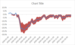
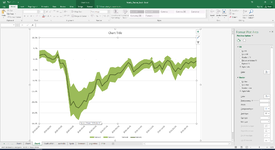
I have a line graph with a range of positive and negative values. Also both hi and low values that I want to shade on both sides of the line graph. The majority of the data points are negative, which made me choose the low value as the stacked area and the high value as the area. Everything below zero turns our how I want it but above zero there is no shaded area, only the line. Any assistance to get the positive values shaded as well would be welcome.
| Weekly_Tracker_Excel.xlsx | ||||||
|---|---|---|---|---|---|---|
| A | B | C | D | |||
| 1 | date | Tracker | Low | High | ||
| 2 | 2020-01-05 | 1.7% | 0.2% | 4.0% | ||
| 3 | 2020-01-12 | 2.2% | 0.9% | 4.2% | ||
| 4 | 2020-01-19 | 2.3% | 0.7% | 4.3% | ||
| 5 | 2020-01-26 | 0.9% | -0.9% | 3.3% | ||
| 6 | 2020-02-02 | 0.5% | -1.2% | 2.6% | ||
| 7 | 2020-02-09 | -0.2% | -2.0% | 1.6% | ||
| 8 | 2020-02-16 | 0.2% | -1.5% | 1.9% | ||
| 9 | 2020-02-23 | 2.2% | 0.4% | 4.3% | ||
| 10 | 2020-03-01 | -2.0% | -4.6% | 0.0% | ||
| 11 | 2020-03-08 | -1.8% | -3.8% | 0.0% | ||
| 12 | 2020-03-15 | -4.1% | -8.0% | -0.5% | ||
| 13 | 2020-03-22 | -13.3% | -17.8% | -6.6% | ||
| 14 | 2020-03-29 | -21.6% | -26.7% | -13.0% | ||
| 15 | 2020-04-05 | -19.6% | -25.4% | -11.1% | ||
| 16 | 2020-04-12 | -22.1% | -27.3% | -13.5% | ||
| 17 | 2020-04-19 | -22.7% | -28.3% | -15.1% | ||
| 18 | 2020-04-26 | -21.2% | -25.0% | -14.6% | ||
| 19 | 2020-05-03 | -19.2% | -23.5% | -13.1% | ||
| 20 | 2020-05-10 | -19.7% | -23.2% | -13.6% | ||
| 21 | 2020-05-17 | -15.9% | -19.4% | -10.5% | ||
| 22 | 2020-05-24 | -15.6% | -18.7% | -10.6% | ||
| 23 | 2020-05-31 | -14.0% | -16.9% | -10.1% | ||
| 24 | 2020-06-07 | -9.4% | -11.8% | -6.1% | ||
| 25 | 2020-06-14 | -9.5% | -13.3% | -5.9% | ||
| 26 | 2020-06-21 | -12.5% | -15.1% | -9.4% | ||
| 27 | 2020-06-28 | -11.0% | -14.5% | -7.9% | ||
| 28 | 2020-07-05 | -10.1% | -13.8% | -7.1% | ||
| 29 | 2020-07-12 | -7.2% | -10.5% | -3.9% | ||
| 30 | 2020-07-19 | -7.2% | -10.7% | -3.7% | ||
| 31 | 2020-07-26 | -7.3% | -10.9% | -4.0% | ||
| 32 | 2020-08-02 | -6.4% | -8.9% | -3.5% | ||
| 33 | 2020-08-09 | -6.3% | -8.8% | -3.8% | ||
| 34 | 2020-08-16 | -5.0% | -7.2% | -2.4% | ||
| 35 | 2020-08-23 | -3.2% | -4.9% | -1.0% | ||
| 36 | 2020-08-30 | -1.5% | -3.3% | 0.5% | ||
| 37 | 2020-09-06 | -2.7% | -5.5% | 0.0% | ||
| 38 | 2020-09-13 | -5.9% | -8.4% | -3.7% | ||
| 39 | 2020-09-20 | -4.8% | -7.2% | -2.4% | ||
| 40 | 2020-09-27 | -4.0% | -6.3% | -1.4% | ||
| 41 | 2020-10-04 | -2.7% | -5.3% | -0.6% | ||
| 42 | 2020-10-11 | -1.9% | -4.3% | 0.0% | ||
| 43 | 2020-10-18 | -1.9% | -4.2% | -0.1% | ||
| 44 | 2020-10-25 | -2.3% | -4.4% | -0.3% | ||
| 45 | 2020-11-01 | -1.1% | -2.8% | 1.1% | ||
| 46 | 2020-11-08 | -4.3% | -6.5% | -1.9% | ||
| 47 | 2020-11-15 | -3.9% | -6.0% | -1.2% | ||
| 48 | 2020-11-22 | -2.6% | -4.7% | -0.6% | ||
| 49 | 2020-11-29 | -4.7% | -7.3% | -1.7% | ||
| 50 | 2020-12-06 | -2.0% | -4.9% | 0.9% | ||
| 51 | 2020-12-13 | -0.5% | -2.8% | 1.7% | ||
| 52 | 2020-12-20 | -1.2% | -3.5% | 0.9% | ||
| 53 | 2020-12-27 | -4.0% | -7.3% | -0.8% | ||
| 54 | 2021-01-03 | -5.8% | -10.0% | -2.7% | ||
| 55 | 2021-01-10 | -4.1% | -6.7% | -1.3% | ||
| 56 | 2021-01-17 | -4.9% | -7.9% | -2.3% | ||
| 57 | 2021-01-24 | -2.9% | -5.5% | -0.4% | ||
| 58 | 2021-01-31 | -1.4% | -3.9% | 0.5% | ||
| 59 | 2021-02-07 | -2.2% | -4.6% | 0.0% | ||
| 60 | 2021-02-14 | -1.1% | -3.2% | 1.0% | ||
| 61 | 2021-02-21 | -1.7% | -4.5% | 0.5% | ||
| 62 | 2021-02-28 | -0.9% | -3.1% | 1.1% | ||
South Africa | ||||||