Hello,
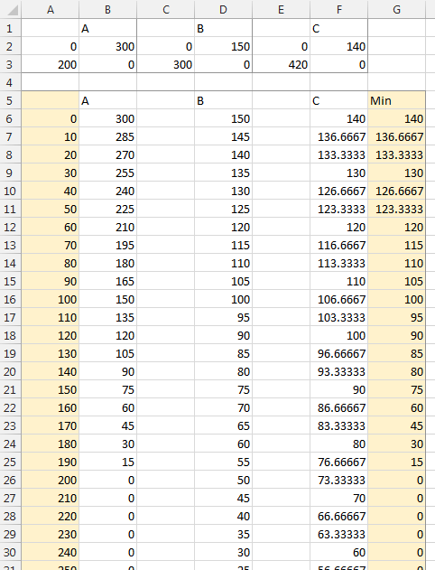
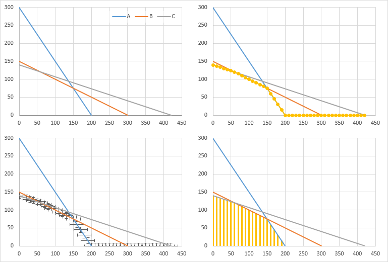
This is probably a simple min/max issue but I have yet to figure it out. My goal is to shade an area below several intersecting lines (feasible region in a group of inequalities). Basically a "fill below" type function but involving several intersecting points (shading below vertices). If you understand linear programming and feasible regions you should have a clear picture of what I'm looking for (intersecting lines, shaded below vertices). Here's an example
 . Let me know if you need the actual chart and formulas I am using. As of now the only way I know how to do this is by using a freeform select and fill. I'm looking for a more automated way such as a formula or chart tool method that will mathematically identify the feasible region and shade it automatically, or a manual input into cells or solver that will shade the chart. Can I use the information from the solver to graph the inequalities AND shade the feasible region? In essence, I want to shade "touching" the chart, or shade it when the chart is created. I'm using XL'10. Thanks in advance.
JV
This is probably a simple min/max issue but I have yet to figure it out. My goal is to shade an area below several intersecting lines (feasible region in a group of inequalities). Basically a "fill below" type function but involving several intersecting points (shading below vertices). If you understand linear programming and feasible regions you should have a clear picture of what I'm looking for (intersecting lines, shaded below vertices). Here's an example
JV
Last edited: