Sheet to Validation as to whether to accept an item from an Outbound Order or not based on the already received return orders

[Sheshashayan M V]

Hi Guys,

I currently have a problem statement that goes like this -
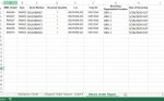
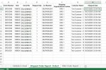
1. There are 2 Excel Workbooks - 1 Sales report (Outbound) & 1 Return Sales report (Inbound). These are for reference & will keep changing every week.
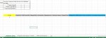
2. Now I have an Invoice that has the Sales Order#, Item ID & Serial number for a said product. Now I need to verify that
a. The details of the above product (as per the invoice) are available in my 1st report (Sales report).
b. The above product (as per the invoice) is not already returned by checking the details of this product with the 2ns report (Return Sales report).

Please refer the attached screenshots for better understanding of the data.

This is an urgent requirement. I tried to learn the relevant topics online to get this done but wasn’t able to do so.
Kindly help, as I have hit the deadline and I need to submit the report on 27th May 2020.

Awaiting your quick & positive response.

Regards,
Sheshashayan M V

 

[Toadstool]

Hi Shesh,

Here's an example but I have it in one workbook, 3 sheets for simplicity. Isn't this just an INDEX MATCH check?
I've let it go "#N/A" so it's obvious when no match is found but you can wrap IFERROR around the formulae with messages for exceptions.
I see all all Qty fields are 1 but I've put a check in cell E2 of Validation just in case more is returned than was ordered.

The Validation sheet just looks for a perfect match of the three specified keys in the two tabs.

SheshashayanMV.xlsx
	A	B	C	D	E	F	G	H
1	Order Number	Item	Serial No.	Shipped Qty	Lot No.	Shipping Org./Location	Customer Name	Shipped Date
2	ORD12310	136253	SRL102267	1	OBLPNSRL1035	ORG 1	Test Cust1	5/21/2020
3	ORD12315	115274	SRL157348	1	OBLPNSRL1444	ORG 1	Test Cust1	5/22/2020
4	ORD12320	194456	SRL145357	1	OBLPNSRL1790	ORG 1	Test Cust1	5/23/2020
5	ORD12325	163640	SRL129803	1	OBLPNSRL1028	ORG 1	Test Cust1	5/24/2020
6	ORD12325	100108	SRL173889	1	OBLPNSRL1455	ORG 1	Test Cust3	5/25/2020
7	ORD12325	187900	SRL105061	1	OBLPNSRL1323	ORG 1	Test Cust3	5/26/2020
8	ORD12340	108825	SRL170520	1	OBLPNSRL1471	ORG 1	Test Cust3	5/27/2020
9	ORD12345	161489	SRL172570	1	OBLPNSRL1495	ORG 1	Test Cust3	5/28/2020
10	ORD12350	101472	SRL138206	1	OBLPNSRL1129	ORG 1	Test Cust3	5/29/2020
11	ORD12355	144562	SRL199134	1	OBLPNSRL1888	ORG 1	Test Cust3	5/30/2020
Shipped

SheshashayanMV.xlsx
	A	B	C	D	E	F	G	H	I
1	RMA Order #	Item	Serial No.	Received Qty	Lot No.	Orig SO	Receiving Org./ Location	Customer Name	Date of Receipt
2	RMA12315	115274	SRL157348	1	OBLPNSRL1444	ORD12315	ORG 1	Test Cust1	5/22/2020
3	RMA12320	194456	SRL145357	1	OBLPNSRL1790	ORD12320	ORG 1	Test Cust1	5/23/2020
4	RMA12325	163640	SRL129803	1	OBLPNSRL1028	ORD12325	ORG 1	Test Cust1	5/24/2020
5	RMA12325	100108	SRL173889	1	OBLPNSRL1455	ORD12325	ORG 1	Test Cust3	5/25/2020
6	RMA12325	187900	SRL105061	1	OBLPNSRL1323	ORD12325	ORG 1	Test Cust3	5/26/2020
7
8
Returns

SheshashayanMV.xlsx
	B	C	D	E	F	G	H	I	J	K	L	M	N	O	P
2	Sales Order	ORD12325
3	Item SKU	163640
4	Item Serial No.	SRL129803
5
6
7	SI No.	Order Number	Item	Serial No.	Shipped Qty	Lot No.	Shipping Org./Location	Customer Name	Shipped Date	Orig SO	RMA Order #	Item	Serial No.	Lot No.	Received Qty
8	1	ORD12325	163640	SRL129803	1	OBLPNSRL1028	ORG 1	Test Cust1	5/24/2020	ORD12325	RMA12325	163640	SRL129803	OBLPNSRL1028	1
9
Validation

Cell Formulas
Range	Formula
E2	E2	=IF(F8-P8<0,"Quantity mismatch","")
C8:J8	C8	=INDEX(Shipped!A2:A9999,MATCH(1,INDEX((Shipped!$A$2:$A$9999=$C$2)*(Shipped!$B$2:$B$9999=$C$3)*(Shipped!$C$2:$C$9999=$C$4),0,1),0))
K8	K8	=INDEX(Returns!F2:F9999,MATCH(1,INDEX((Returns!$F$2:$F$9999=$C$2)*(Returns!$B$2:$B$9999=$C$3)*(Returns!$C$2:$C$9999=$C$4),0,1),0))
L8:N8	L8	=INDEX(Returns!A2:A9999,MATCH(1,INDEX((Returns!$F$2:$F$9999=$C$2)*(Returns!$B$2:$B$9999=$C$3)*(Returns!$C$2:$C$9999=$C$4),0,1),0))
O8	O8	=INDEX(Returns!E2:E9999,MATCH(1,INDEX((Returns!$F$2:$F$9999=$C$2)*(Returns!$B$2:$B$9999=$C$3)*(Returns!$C$2:$C$9999=$C$4),0,1),0))
P8	P8	=INDEX(Returns!D2:D9999,MATCH(1,INDEX((Returns!$F$2:$F$9999=$C$2)*(Returns!$B$2:$B$9999=$C$3)*(Returns!$C$2:$C$9999=$C$4),0,1),0))