Hi All,
Please see attached spreadsheet.
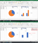
I have a pivot pie chart chart with 2 categories and a slicer.
In the overview of the pie chart, Category 1 is in blue and Category 2 is in orange color.
However, when i use the slicer (Category) to filter to Category 2 (alone), the pie of Category 2 is shown as blue instead of orange. I thought this was weird so i recolored the pie again:
1) colored Category 2 pie to Orange using format/shape fill at top menu AND using the data point side panel (just to be safe)
2) I cleared the filter on the slicer, filtered again to Category 2 and it worked - the Category 2 pie was in Orange
However, when i restart my workbook, used the slicer to filter to category 2, the Category 2 pie turned back to Blue.
Please can i seek your advice on this issue? How can i maintain the color format for Category 2?
Thank you!
Please see attached spreadsheet.
I have a pivot pie chart chart with 2 categories and a slicer.
In the overview of the pie chart, Category 1 is in blue and Category 2 is in orange color.
However, when i use the slicer (Category) to filter to Category 2 (alone), the pie of Category 2 is shown as blue instead of orange. I thought this was weird so i recolored the pie again:
1) colored Category 2 pie to Orange using format/shape fill at top menu AND using the data point side panel (just to be safe)
2) I cleared the filter on the slicer, filtered again to Category 2 and it worked - the Category 2 pie was in Orange
However, when i restart my workbook, used the slicer to filter to category 2, the Category 2 pie turned back to Blue.
Please can i seek your advice on this issue? How can i maintain the color format for Category 2?
Thank you!