etaf
Well-known Member
- Joined
- Oct 24, 2012
- Messages
- 8,271
- Office Version
- 365
- Platform
- MacOS
I have had some help here previously, but using 365 functions and the solutions have been great
However , now i'm trying to use 2019 version functions only
The person i'm helping is very pleased with the functionality of the 365 version , And in US I'm in UK - so a bit of a timezone issue
BUT last weekend they upgraded to the online model - and have been told the online version is 2019 and the desktop app is 365 , so when they are online, they get a #NAME error
They have flagged with IT that this is a major compatibility issue and will impact a lot of people , but this is the first issue - they may sort out in few weeks
Does not make sense to me, as I was under the impression all online was now 365, various subscriptions for Business
She has the Apps on the desktop still 365 version and online 2019 version to share with other workers
But she gets a #NAME error for any 365 functions I have used !!!!!!! - Textbefore() & filter() , LET() etc
I have updated the formulas to use ONLY 2019 versions - BUT she also wants to sort the summary extraction by the NAME , which is not working - Looks up and returns the same order of name in the list , unless the source data is sorted, which they do not want to do - It maybe not possible, which is fine
In my example - just for clarity
I have 2 helper columns AA and AB
AA is just to get the 1st line of a cell - as the main one will have a lot of char(10) - so thats AA , just the first line, and i can pull the data from that column
Then we have a criteria to show only rows below a certain % based on column P - BUT i could not make that work - so i have another helper column AB which simply uses the <=% in the summary and flags the row as a 1
so i then use the 1 as a criteria in that column AB to pull over the rows i need - Those 2 columns are also in a table because , she deletes rows and inserts rows - to archive info
And that took a lot of thought as I'm so used to the easier functions now in 365
I have used
=IFERROR(INDEX(Active!$AA$2:$AA$500,SMALL(IF(Active!$AB$2:$AB$500=1,ROW($K$2:$K$500)),ROW(1:1))-1,1),"")
to Pull out the name in column AA , based on the criteria of a 1 in AB column
This works fine and pulls out the names
Then I use
=IF($E3="","",INDEX(Active!K$2:K$500,MATCH(Summary!$E3,Active!$AA$2:$AA$500,0)))
to lookup column K based on the name
I know there will be an issue if the same name is duplicated , and the wrong info will be pulled over , but that does seem to be a high risk , and WIP for a unique ID for each row
Then I use the same formula in the other columns on summary to pull over the other columns needed
Everything works fine
UNTIL
The Summary sheet cannot be sorted - as the names remain in the same order , they are in the data sheet , but the other columns do sort and so the WRONG associated data is extracted
I know she should probably sort the raw data sheet , and then the names will be extracted in the correct order
BUT wondered if there was a formula to replace
=IFERROR(INDEX(Active!$AA$2:$AA$500,SMALL(IF(Active!$AB$2:$AB$500=1,ROW($K$2:$K$500)),ROW(1:1))-1,1),"")
I have used google and searched various forums , also looking through all my previous examples
Problem now of course with FILTER being available from 2021 version and 365 - MOST google results tend to show 365 functions
I did come across a couple of other formulas - BUT they work the same - looking at the rows, so bring back in order on data sheet
maybe its NOT possible to do this just in the summary and the only way is the Data sheet being sorted, which is fine, if thats the reality
DATA SHEET - named ACTIVE
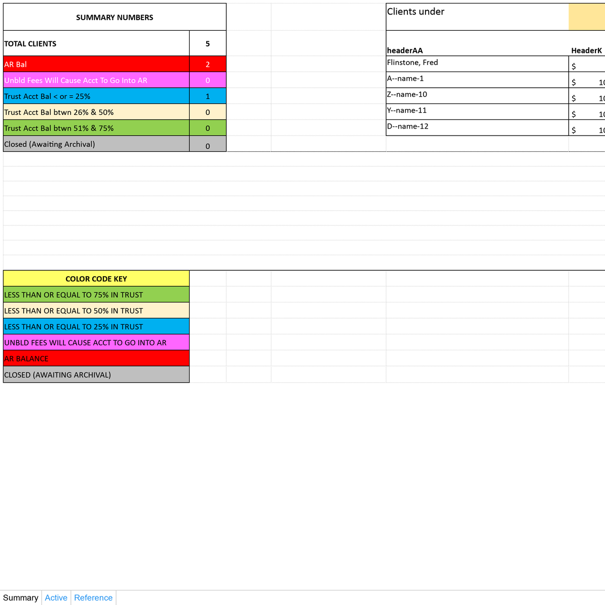
SUMMARY SHEET
I only leave the file on the share for a fewdays
However , now i'm trying to use 2019 version functions only
The person i'm helping is very pleased with the functionality of the 365 version , And in US I'm in UK - so a bit of a timezone issue
BUT last weekend they upgraded to the online model - and have been told the online version is 2019 and the desktop app is 365 , so when they are online, they get a #NAME error
They have flagged with IT that this is a major compatibility issue and will impact a lot of people , but this is the first issue - they may sort out in few weeks
Does not make sense to me, as I was under the impression all online was now 365, various subscriptions for Business
She has the Apps on the desktop still 365 version and online 2019 version to share with other workers
But she gets a #NAME error for any 365 functions I have used !!!!!!! - Textbefore() & filter() , LET() etc
I have updated the formulas to use ONLY 2019 versions - BUT she also wants to sort the summary extraction by the NAME , which is not working - Looks up and returns the same order of name in the list , unless the source data is sorted, which they do not want to do - It maybe not possible, which is fine
In my example - just for clarity
I have 2 helper columns AA and AB
AA is just to get the 1st line of a cell - as the main one will have a lot of char(10) - so thats AA , just the first line, and i can pull the data from that column
Then we have a criteria to show only rows below a certain % based on column P - BUT i could not make that work - so i have another helper column AB which simply uses the <=% in the summary and flags the row as a 1
so i then use the 1 as a criteria in that column AB to pull over the rows i need - Those 2 columns are also in a table because , she deletes rows and inserts rows - to archive info
And that took a lot of thought as I'm so used to the easier functions now in 365
I have used
=IFERROR(INDEX(Active!$AA$2:$AA$500,SMALL(IF(Active!$AB$2:$AB$500=1,ROW($K$2:$K$500)),ROW(1:1))-1,1),"")
to Pull out the name in column AA , based on the criteria of a 1 in AB column
This works fine and pulls out the names
Then I use
=IF($E3="","",INDEX(Active!K$2:K$500,MATCH(Summary!$E3,Active!$AA$2:$AA$500,0)))
to lookup column K based on the name
I know there will be an issue if the same name is duplicated , and the wrong info will be pulled over , but that does seem to be a high risk , and WIP for a unique ID for each row
Then I use the same formula in the other columns on summary to pull over the other columns needed
Everything works fine
UNTIL
The Summary sheet cannot be sorted - as the names remain in the same order , they are in the data sheet , but the other columns do sort and so the WRONG associated data is extracted
I know she should probably sort the raw data sheet , and then the names will be extracted in the correct order
BUT wondered if there was a formula to replace
=IFERROR(INDEX(Active!$AA$2:$AA$500,SMALL(IF(Active!$AB$2:$AB$500=1,ROW($K$2:$K$500)),ROW(1:1))-1,1),"")
I have used google and searched various forums , also looking through all my previous examples
Problem now of course with FILTER being available from 2021 version and 365 - MOST google results tend to show 365 functions
I did come across a couple of other formulas - BUT they work the same - looking at the rows, so bring back in order on data sheet
maybe its NOT possible to do this just in the summary and the only way is the Data sheet being sorted, which is fine, if thats the reality
DATA SHEET - named ACTIVE
| Wayne FORUM Help2.xlsx | ||||||||||||||||||||||||||||||
|---|---|---|---|---|---|---|---|---|---|---|---|---|---|---|---|---|---|---|---|---|---|---|---|---|---|---|---|---|---|---|
| A | K | L | M | N | O | P | Z | AA | AB | |||||||||||||||||||||
| 1 | HeaderA | HeaderK | headerL | Header M | Header N | Header O | Header P | HeaderAA | Below threshold | |||||||||||||||||||||
| 2 | Flinstone, Fred 123456789 abced ef g | $2,000.00 | $0.00 | $20.00 | $200.00 | $2,220.00 | -11.000% | Flinstone, Fred | 1 | |||||||||||||||||||||
| 3 | A--name-1 -------2nd line | $10,000.00 | $9,000.00 | $10.00 | $0.00 | $1,010.00 | 89.900% | A--name-1 | 1 | |||||||||||||||||||||
| 4 | Z--name-10 ------ line 2 | $10,000.00 | $10,000.00 | $0.00 | $0.00 | $0.00 | 100.000% | Z--name-10 | 1 | |||||||||||||||||||||
| 5 | Y--name-11 ------- line 2 ---------line 3 | $10,000.00 | $2,300.00 | $0.00 | $0.00 | $7,700.00 | 23.000% | Y--name-11 | 1 | |||||||||||||||||||||
| 6 | D--name-12 | $10,000.00 | $0.00 | $0.00 | $12.00 | $10,012.00 | -0.120% | D--name-12 | 1 | |||||||||||||||||||||
Active | ||||||||||||||||||||||||||||||
| Cell Formulas | ||
|---|---|---|
| Range | Formula | |
| O2:O6 | O2 | =IF(A2="","",SUM(K2)-(L2-M2)+(N2)) |
| P2:P6 | P2 | =IFERROR(IF(K2="Closed","Closed",((L2-M2-N2)/K2)),"") |
| AA2:AA6 | AA2 | =IF(A2="","",IFERROR(LEFT(A2,FIND(CHAR(10),A2,1)),A2)) |
| AB2:AB6 | AB2 | =IF(A2="","",IF(P2<=Summary!$F$1/100,1,0)) |
| Cells with Conditional Formatting | ||||
|---|---|---|---|---|
| Cell | Condition | Cell Format | Stop If True | |
| L2:O19,L21:O500 | Expression | =$K2="closed" | text | NO |
| A2:Q19,A21:Q500,A20:J20,Q20 | Expression | =$P2="closed" | text | YES |
| A2:Q19,A20:J20,Q20,A21:Q500 | Expression | =$N2>0 | text | YES |
| A2:Q19,A20:J20,Q20,A21:Q500 | Expression | =AND($L2<>"",($L2-$M2)<=0) | text | NO |
| A2:Q19,A20:J20,Q20,A21:Q500 | Expression | =AND($P2<>"",$P2<=0.25) | text | NO |
| A2:Q19,A20:J20,Q20,A21:Q500 | Expression | =AND($P2<>"",$P2<=0.5) | text | NO |
| A2:Q19,A20:J20,Q20,A21:Q500 | Expression | =AND($P2<>"",$P2<=0.75) | text | NO |
SUMMARY SHEET
| Wayne FORUM Help2.xlsx | |||||||||
|---|---|---|---|---|---|---|---|---|---|
| E | F | G | H | I | J | K | |||
| 1 | Clients under | 100% | <- enter the Number - NOT a Percent - EG for 35%, just type in 35 - Trust Balance to Minimum Retainer % required to extract the summary below | ||||||
| 2 | headerAA | HeaderK | headerL | Header M | Header N | Header O | Header P | ||
| 3 | Flinstone, Fred | $ 2,000.00 | $ - | $ 20.00 | $ 200.00 | $ 2,220.00 | -11% | ||
| 4 | A--name-1 | $ 10,000.00 | $ 9,000.00 | $ 10.00 | $ - | $ 1,010.00 | 90% | ||
| 5 | Z--name-10 | $ 10,000.00 | $ 10,000.00 | $ - | $ - | $ - | 100% | ||
| 6 | Y--name-11 | $ 10,000.00 | $ 2,300.00 | $ - | $ - | $ 7,700.00 | 23% | ||
| 7 | D--name-12 | $ 10,000.00 | $ - | $ - | $ 12.00 | $ 10,012.00 | 0% | ||
Summary | |||||||||
| Cell Formulas | ||
|---|---|---|
| Range | Formula | |
| E3:E7 | E3 | =IFERROR(INDEX(Active!$AA$2:$AA$500,SMALL(IF(Active!$AB$2:$AB$500=1,ROW($K$2:$K$500)),ROW(1:1))-1,1),"") |
| F3:K7 | F3 | =IF($E3="","",INDEX(Active!K$2:K$500,MATCH(Summary!$E3,Active!$AA$2:$AA$500,0))) |
| Cells with Conditional Formatting | ||||
|---|---|---|---|---|
| Cell | Condition | Cell Format | Stop If True | |
| E3:K9,E15:K201,E10:E14 | Expression | =$E3<>"" | text | NO |
I only leave the file on the share for a fewdays
Last edited:
")


