searchingforhelp
Board Regular
- Joined
- Nov 11, 2020
- Messages
- 67
- Office Version
- 365
- Platform
- Windows
Hi, I hope all is well.
Need assistance with two separate formulas
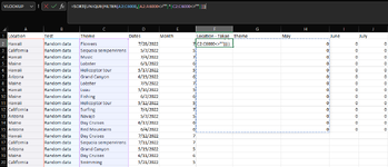
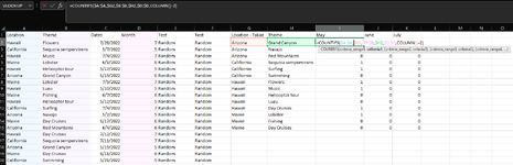
1. There are a total of four locations listed in column A. I am trying to separate the locations and identify the theme with that location, and the number of times it occurred in a specified month. I am only able to identify the theme in column F and the monthly occurrence in column G, H and I but not the location. Looking for a formula that will provide me the location with the theme and column G, H and I. Something similar to the attached image if applicable. Please note the list is longer in Column A, in case you are wondering why the numbers are not adding up
2. Is there a way to simplify the formula in column G, H and I from the data listed in column C rather than using column D?
 . .
. .
Need assistance with two separate formulas
1. There are a total of four locations listed in column A. I am trying to separate the locations and identify the theme with that location, and the number of times it occurred in a specified month. I am only able to identify the theme in column F and the monthly occurrence in column G, H and I but not the location. Looking for a formula that will provide me the location with the theme and column G, H and I. Something similar to the attached image if applicable. Please note the list is longer in Column A, in case you are wondering why the numbers are not adding up
2. Is there a way to simplify the formula in column G, H and I from the data listed in column C rather than using column D?
. .| Mr Excel.xlsx | |||||||||||
|---|---|---|---|---|---|---|---|---|---|---|---|
| A | B | C | D | E | F | G | H | I | |||
| 1 | Location | Theme | Dates | Month | Theme | May | June | July | |||
| 2 | Hawaii | Flowers | 7/28/2022 | Jul | Day Cruises | 0 | 2 | 1 | |||
| 3 | California | Sequoia sempervirens | 5/7/2022 | May | Fishing | 0 | 1 | 0 | |||
| 4 | Hawaii | Music | 7/4/2022 | Jul | Flowers | 0 | 0 | 1 | |||
| 5 | Maine | Lobster | 6/1/2022 | Jun | Grand Canyon | 1 | 1 | 0 | |||
| 6 | Hawaii | Helicoptor tour | 5/17/2022 | May | Helicoptor tour | 2 | 0 | 0 | |||
| 7 | Arizona | Grand Canyon | 6/19/2022 | Jun | Lobster | 0 | 1 | 1 | |||
| 8 | Maine | Lobster | 7/9/2022 | Jul | Luau | 1 | 0 | 0 | |||
| 9 | Hawaii | Luau | 5/10/2022 | May | Music | 0 | 0 | 1 | |||
| 10 | Maine | Fishing | 6/7/2022 | Jun | Navajo | 1 | 0 | 0 | |||
| 11 | Hawaii | Helicoptor tour | 5/12/2022 | May | Red Mountains | 0 | 1 | 0 | |||
| 12 | California | Surfing | 7/4/2022 | Jul | Sequoia sempervirens | 1 | 0 | 1 | |||
| 13 | Arizona | Navajo | 5/7/2022 | May | Surfing | 0 | 0 | 1 | |||
| 14 | Maine | Day Cruises | 6/17/2022 | Jun | Swimming | 1 | 0 | 0 | |||
Sheet1 | |||||||||||
| Cell Formulas | ||
|---|---|---|
| Range | Formula | |
| F2:F14 | F2 | =SORT(UNIQUE(FILTER(B2:B6000,B2:B6000<>""))) |
| G2:G14 | G2 | =COUNTIFS(B:B,F2#,D:D,"May") |
| H2:H14 | H2 | =COUNTIFS(B:B,F2#,D:D,"Jun") |
| I2:I14 | I2 | =COUNTIFS(B:B,F2#,D:D,"Jul") |
| D2:D14 | D2 | =CHOOSE((MONTH(C2)),"Jan","Feb","Mar","Apr","May","Jun","Jul","Aug","Sep","Oct","Nov","Dec") |
| Dynamic array formulas. | ||
")