#Spill Error fixes

[captjakku]

Hi,

I am working within a very large workbook and using the index function to grab ranges of amounts and corresponding dates from many different sheets. This generates the list I need and is exactly what I want. The issue I am having is the recognition that as new rows are added to the sheets in the future, this will break the list as a new row within the range with result in a spill error. The perfect fix would be to have a function that adds a new row(s) to the list to accommodate the dynamic range, but I know nothing about macros. There is also way too many ranges that I am indexing to list them horizontally.

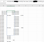
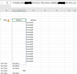
The first picture is a snip of the list, a dynamic range with another dynamic range underneath and so on. The second picture is what happens when I essentially increase the size of the dynamic range by adding a row to the corresponding sheet for an additional entry.

Basically I am in need of a way to index many different ranges and have the resulting dynamic ranges not interfere with each other. I was hoping some brilliant person on here has a suggestion to fix or an alternative to achieve what I want. Thanks so much for your time.

 

[awoohaw]

you have 365. you may be able to build all of your formulas with a LET statement, including the rows that are supposed to be below the #SPILL Range.
LET(a, TheFormulaToCreateSpillRange, b, the formulas for the rows below, VSTACK(a,b))

 

[Peter_SSs]

build all of your formulas with a LET statement,

It could be done that way but it could also just be done directly with VSTACK

=VSTACK(FormulaForFirstDynamicRange,FormulaForSecondDynamicRange,FormulaForThirdDynamicRange, . . . .)

@captjakku
Note that both these options will only work as-is if all dynamic arrays contain the same number of columns (in this case one column from the appearance of your images).

 

[captjakku]

It could be done that way but it could also just be done directly with VSTACK

=VSTACK(FormulaForFirstDynamicRange,FormulaForSecondDynamicRange,FormulaForThirdDynamicRange, . . . .)

@captjakku
Note that both these options will only work as-is if all dynamic arrays contain the same number of columns (in this case one column from the appearance of your images).

VSTACK worked really well, thank you so much!

 

[Peter_SSs]

You're welcome. Glad we could help. Thanks for the follow-up.