#Spill! Error when trying to find average of 2 letter grades

[photogfrog]

Good afternoon;

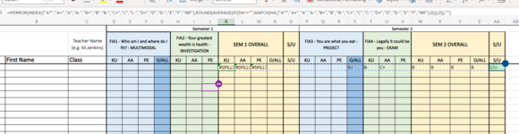
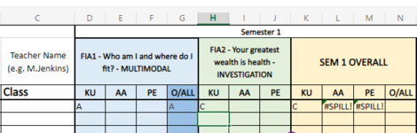
I'm trying to get 2 cells, not side-by-side, to average 2 letter grades in a 3rd cell. All I am getting is a #Spill! error.
Also, if I do enter grades into the cells, it subs the value in H4 into K4, which is not helpful as it is not finding the average. In my screenshot, it should be a B, but it's taking the C only.
The formula currently in K4 is =IFERROR(INDEX({"A*","A+","A","A-","B+","B","B-","C+","C","C-","D+","D","D-","E","F","NR"},ROUND(AVERAGE(IF(D4<>"",MATCH(H4,{"A*","A+","A","A-","B+","B","B-","C+","C","C-","D+","D","D-","E","F","NR"},0))),0)),"")

Help please and many many thanks in advance.

 

[Peter_SSs]

Welcome to the MrExcel board!

See if either of these does what you want. Col K is if you have the LET function in your MS365. Col L is the same formula but without the LET function.

If this is not what you want then please explain in words what should happen for each of my sample cases (or your own other sample cases)

BTW, are columns D & H manually entered or do they contain formulas?

21 12 01.xlsm
	D	E	F	G	H	I	J	K	L
4	A				C			B	B
5	B							B	B
6					D			D	D
7
8	A-				D+			C+	C+
9	A*				F			C+	C+
Sheet2 (2)

Cell Formulas
Range	Formula
K4:K9	K4	=LET(grades,{"A*","A+","A","A-","B+","B","B-","C+","C","C-","D+","D","D-","E","F","NR"}, IF(COUNTA(D4,H4)=2,INDEX(grades,ROUND(AVERAGE(MATCH(D4,grades,0),MATCH(H4,grades,0)),0)),D4&H4))
L4:L9	L4	=IF(COUNTA(D4,H4)=2,INDEX({"A*","A+","A","A-","B+","B","B-","C+","C","C-","D+","D","D-","E","F","NR"},ROUND(AVERAGE( MATCH(D4,{"A*","A+","A","A-","B+","B","B-","C+","C","C-","D+","D","D-","E","F","NR"},0), MATCH(H4,{"A*","A+","A","A-","B+","B","B-","C+","C","C-","D+","D","D-","E","F","NR"},0)),0)),D4&H4)

 

[photogfrog]

D and H are manually entered grades.

 

[photogfrog]

omg omg o

Welcome to the MrExcel board!

See if either of these does what you want. Col K is if you have the LET function in your MS365. Col L is the same formula but without the LET function.

If this is not what you want then please explain in words what should happen for each of my sample cases (or your own other sample cases)

BTW, are columns D & H manually entered or do they contain formulas?

21 12 01.xlsm
	D	E	F	G	H	I	J	K	L
4	A				C			[FORMULA='=LET(grades,{"A*","A+","A","A-","B+","B","B-","C+","C","C-","D+","D","D-","E","F","NR"},
Sheet2 (2)

21 12 01.xlsm
OMG! THAT WORKED! THANK YOU SO MUCH!!!! :) :)
Sheet2 (2)

 

[Peter_SSs]

D and H are manually entered grades.

OK, thanks

THAT WORKED! THANK YOU SO MUCH!!!!

You're welcome. Glad we could help. Thanks for the follow-up.