Hello all,
This is my first post here so hello everyone, pleased to meet you all") I'm a self taught Excel user so my skills at this stage are unfortunately a bit limited and quite rough on the edges as well.
I'm a self taught Excel user so my skills at this stage are unfortunately a bit limited and quite rough on the edges as well.
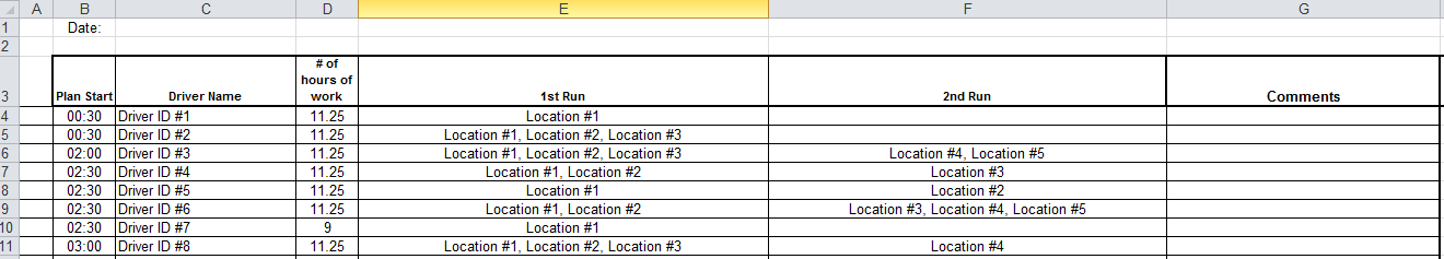
I recently started working for a new company and I'm working on a spreadsheet that'll make my and my colleagues lives easier. We've got a sheet with driver names and the delivery locations. Until now, the guys here were retyping all the locations manually from another spreadsheet and matching them to the appropriate driver for the particular day. It looks like this:
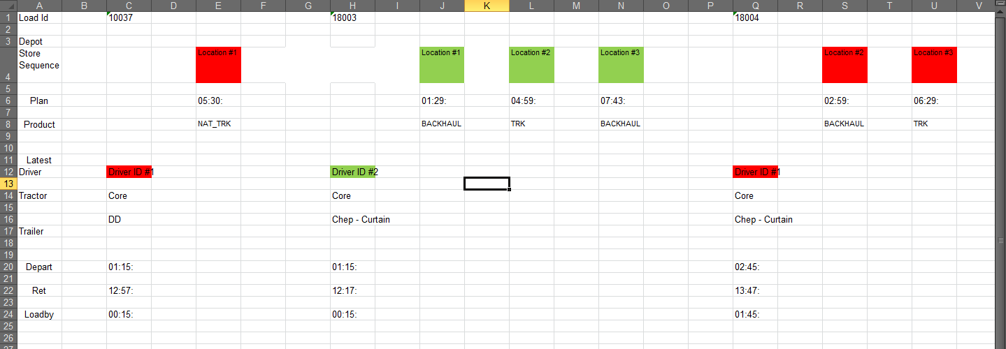
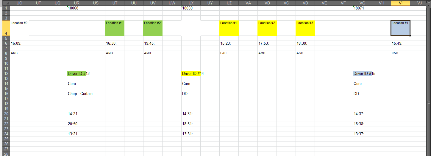
The database from the other spreadsheet, after being pasted into an additional sheet in the file from the screen shot up looks like this:
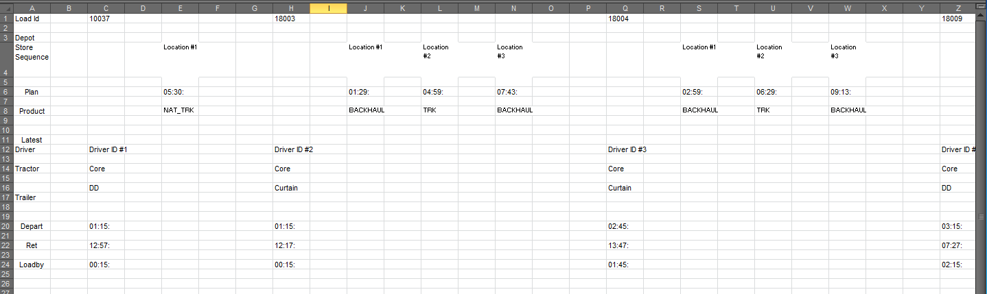
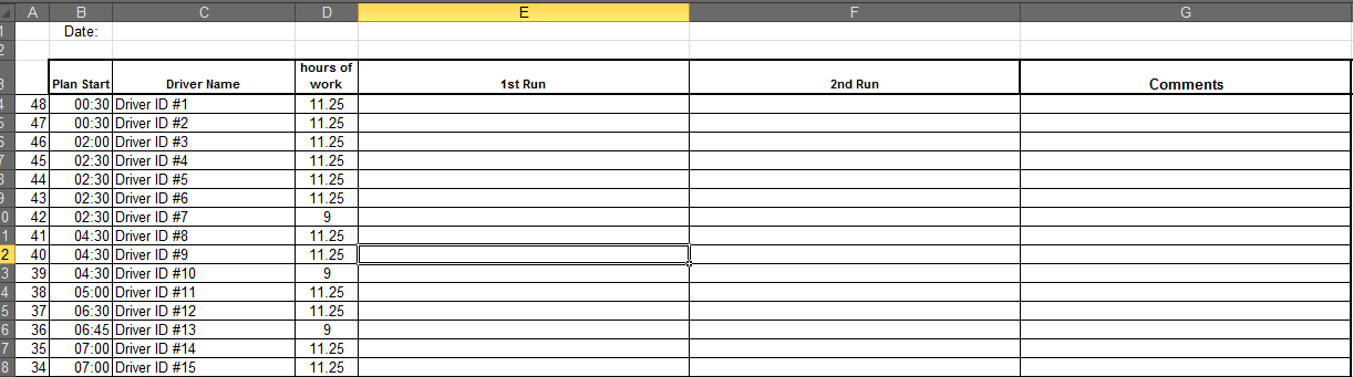
What I want the spreadsheet to do is that you copy the database into a blank sheet in the file and it automatically fills itself in with the correct locations to the appropriate drivers. I was thinking of using the formulas INDEX and MATCH, but I am not sure how to modify the formula in order for it to find the data I want. When I use =INDEX(Sheet1!$4:$4,MATCH('Driver Names'!C4,Sheet1!$12:$12,0)) it sends me directly above the Driver ID in the database sheet and I want it to find the data 2 cells to the right instead. There is also a possibility for a driver to have several locations for 1 run, which means probably the IF formula, that IF the cell 2 cells to the right is full then return the value in the same cell after a coma, for example. I figured that the CONCATENATE formula might come in place in this instance, but I am really clueless how to make it all work together nice and tidily. There are also 2nd runs for drivers, which means the same name is going to appear in the database sheet 2x, so I guess the IF function again for if the 1st RUN cell is filled in with a location already then find another same Diver ID in the sheet and use the 2nd data and not the 1st one. It is a really complicated spreadsheet for me and I need some guidance from you guys. I'm still learning the arts of Excel so please forgive my noobness If anything is not clear or my explanation seems a bit off, please don't hesitate to ask me for clarification.
Thanks in advance for any advice!
This is my first post here so hello everyone, pleased to meet you all
I'm a self taught Excel user so my skills at this stage are unfortunately a bit limited and quite rough on the edges as well.I recently started working for a new company and I'm working on a spreadsheet that'll make my and my colleagues lives easier. We've got a sheet with driver names and the delivery locations. Until now, the guys here were retyping all the locations manually from another spreadsheet and matching them to the appropriate driver for the particular day. It looks like this:
The database from the other spreadsheet, after being pasted into an additional sheet in the file from the screen shot up looks like this:
What I want the spreadsheet to do is that you copy the database into a blank sheet in the file and it automatically fills itself in with the correct locations to the appropriate drivers. I was thinking of using the formulas INDEX and MATCH, but I am not sure how to modify the formula in order for it to find the data I want. When I use =INDEX(Sheet1!$4:$4,MATCH('Driver Names'!C4,Sheet1!$12:$12,0)) it sends me directly above the Driver ID in the database sheet and I want it to find the data 2 cells to the right instead. There is also a possibility for a driver to have several locations for 1 run, which means probably the IF formula, that IF the cell 2 cells to the right is full then return the value in the same cell after a coma, for example. I figured that the CONCATENATE formula might come in place in this instance, but I am really clueless how to make it all work together nice and tidily. There are also 2nd runs for drivers, which means the same name is going to appear in the database sheet 2x, so I guess the IF function again for if the 1st RUN cell is filled in with a location already then find another same Diver ID in the sheet and use the 2nd data and not the 1st one. It is a really complicated spreadsheet for me and I need some guidance from you guys. I'm still learning the arts of Excel so please forgive my noobness
If anything is not clear or my explanation seems a bit off, please don't hesitate to ask me for clarification.Thanks in advance for any advice!