Spreadsheet to keep track of my daily walking time

[Burrgogi]

Hello everyone! I've gained some weight recently and so I've started a daily walking routine that will hopefully shed some of the excess weight. I've got 3 different walking routes that I like to take, A, B & C.
A= 30 min
B= 38 min
C= 45 min
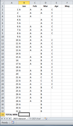
As you can see from my spreadsheet, I've put the corresponding letter to each day of the month. I don't know how to tally up the total number of minutes that correspond to those letters.

Secondly, there are days when I put in 2 walking sessions per day. (e.g. A + A = 60 min). I don't know how to account for that in my setup.

There are also days when I don't do any walking but rather bicycling and they don't fit into any pattern (routes A, B or C). So I guess I need some flexibility in the worksheet to manually type in the number of minutes (e.g. 1 hr 10 min). Any ideas on all this?

 

[PuntingJawa]

I hope you don't mind but I mocked something up. I added "Time" Lines next to the letter ones. Linked using "IF" formulas to link A to 30 B to 38 and C to 45. Then linked cells together that would allow it to auto calculate each month from the numbers and also a Total for the year at the end linking the linked cells to one another.

Tracking RouteA to RouteC.xlsx
	A	B	C	D	E	F	G	H	I	J	K	L	M	N	O	P	Q	R	S	T	U	V	W	X	Y
1	Day	Jan	Time	Feb	Time	Mar	Time	Apr	Time	May	Time	Jun	Time	Jul	Time	Aug	Time	Sep	Time	Oct	Time	Nov	Time	Dec	Time
2	1	a	30	a	30
3	2			a	30
4	3	a	30	a	30
5	4	a	30
6	5	a	30
7	6	a	30	a	30
8	7	a	30	a	30
9	8	a	30	a	30
10	9	a	30	a	30
11	10	a	30	a	30
12	11	a	30	a	30
13	12	a	30	a	30
14	13	a	30	a	30
15	14	a	30
16	15	a	30	a	30
17	16			a	30
18	17	a	30	a	30
19	18	a	30
20	19	a	30	a	30
21	20			a	30
22	21	a	30	a	30
23	22	a	30	a	30
24	23	a	30	a	30
25	24	a	30	a	30
26	25	a	30	a	30
27	26	a	30	a	30
28	27	a	30	a	30
29	28	a	30	a	30
30	29	a	30	a	30
31	30	a	30
32	31	a	30
33	Totals		840	Minutes	750		0		0		0		0		0		0		0		0		0		0
34																								Total	1590
Sheet1

Cell Formulas
Range	Formula
C2:C32,Y2:Y32,W2:W32,U2:U32,S2:S32,Q2:Q32,O2:O32,M2:M32,K2:K32,I2:I32,G2:G32,E2:E32	C2	=IF(B2="A",30,IF(B2="B",38,IF(B2="C",45,"")))
C33,Y33,W33,U33,S33,Q33,O33,M33,K33,I33,G33,E33	C33	=SUM(C2:C32)
Y34	Y34	=SUM(C33,E33,G33,I33,K33,M33,O33,Q33,S33,U33,W33,Y33)

 

[Fluff]

I suggest that you update your Account details (or click your user name at the top right of the forum) so helpers always know what Excel version(s) & platform(s) you are using as the best solution often varies by version. (Don’t forget to scroll down & ‘Save’)

Another option

+Fluff 1.xlsm
	A	B
1
2	1	A
3	2	A
4	3	A
5	4	A
6	5	A
7	6
8	7	B
9	8	A
10	9	A
11	10	B
12	11	A
13	12
14	13	A
15	14	C
16	15	A
17	16	60
18	17	A
19	18
20	19	A
21	20	A
22	21	45
23	22	A
24	23
25	24	A
26	25	A
27	26
28	27	A
29	28	A
30	29	A
31	30	A
32	31
33		821
Master

Cell Formulas
Range	Formula
A2:A32	A2	=SEQUENCE(31)
B33	B33	=SUMPRODUCT(((B2:B32="A")*30)+((B2:B32="B")*38)+((B2:B32="C")*40))+SUM(B2:B32)
Dynamic array formulas.

 

[petertenthije]

Using the setup prodvided byy PuntingJawa, you can replace the formula in C2 by:

=SUMPRODUCT(LEN(D2)-LEN(SUBSTITUTE(D2;"A";"")))*30+SUMPRODUCT(LEN(D2)-LEN(SUBSTITUTE(D2;"B";"")))*38+SUMPRODUCT(LEN(D2)-LEN(SUBSTITUTE(D2;"C";"")))*45

In that case you can type AAB in one cell and it will count 30+30+38=98.


Edited to add:
Depending on your Excel settings you might have to change the semicolons into commas!
=SUMPRODUCT(LEN(D2)-LEN(SUBSTITUTE(D2,"A","")))*30+SUMPRODUCT(LEN(D2)-LEN(SUBSTITUTE(D2,"B","")))*38+SUMPRODUCT(LEN(D2)-LEN(SUBSTITUTE(D2,"C","")))*45

 

[PuntingJawa]

Using what @petertenthije did it looks like this

Tracking RouteA to RouteC.xlsx
	A	B	C	D	E	F	G
1	Day	Jan	Time	Feb	Time	Mar	Time
2	1	A B C	113		0		0
3	2	A B	68		0		0
4	3	A C	75		0		0
5	4	B C	83		0		0
6	5	ABC	113		0		0
7	6	AB	68		0		0
8	7	AC	75		0		0
9	8	BC	83		0		0
10	9		0		0		0
11	10		0		0		0
12	11		0		0		0
13	12		0		0		0
14	13		0		0		0
15	14		0		0		0
16	15		0		0		0
17	16		0		0		0
18	17		0		0		0
19	18		0		0		0
20	19		0		0		0
21	20		0		0		0
22	21		0		0		0
23	22		0		0		0
24	23		0		0		0
25	24		0		0		0
26	25		0		0		0
27	26		0		0		0
28	27		0		0		0
29	28		0		0		0
30	29		0		0		0
31	30		0		0		0
32	31		0		0		0
33	Totals		678		0		0
34
35		Routes			Format
36		A-30 Minutes			Both ABC and A B C will work
37		B-38 Minutes			Use all capital letters
38		C-45 Minutes			Lowercase will bring 0
Sheet1

Cell Formulas
Range	Formula
C2:C32,G2:G32,E2:E32	C2	=SUMPRODUCT(LEN(B2)-LEN(SUBSTITUTE(B2,"A","")))*30+SUMPRODUCT(LEN(B2)-LEN(SUBSTITUTE(B2,"B","")))*38+SUMPRODUCT(LEN(B2)-LEN(SUBSTITUTE(B2,"C","")))*45
C33,G33,E33	C33	=SUM(C2:C32)

Unlike with mine that can use both A a B b C c this one needs all capital letters. However I did miss you saying that you do multiple routes sometimes and mine didn't allow that. I used the edited version they posted with "," instead of ";" and tested. The example above shows it works with both spaces and together.

 

[Fluff]

Same idea but without helper columns

=SUMPRODUCT(((LEN(B2:B32)-LEN(SUBSTITUTE(B2:B32,"A","")))*30)+((LEN(B2:B32)-LEN(SUBSTITUTE(B2:B32,"B","")))*38)+((LEN(B2:B32)-LEN(SUBSTITUTE(B2:B32,"C","")))*40))+SUM(B2:B32)

 

[Fluff]

Slightly shorter depending on version

=SUM(FILTERXML("<k>"&SUBSTITUTE(SUBSTITUTE(SUBSTITUTE(TEXTJOIN(,,B2:B32),"A","<x>30</x>"),"B","<x>38</x>"),"C","<x>40</x>")&"</k>","//x"))+SUM(B2:B32)