Struggling with conditions of IF statements

heathermchle

New Member
Joined
Jun 7, 2022
Messages
15
Office Version
  1. 2010
Platform
  1. Windows
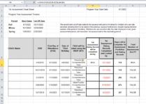
Hi, I'm working on an interactive spread sheet to use with the teachers that I support and I'm trying to find a way to make the cells in one column display certain text based on the conditions in another. I've literally spent the equivalent of two work days, it feels like, playing with formulas, trying different things. I KNOW there is a way but I just can't figure it out! Spreadsheet is below:

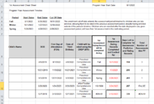
The user will input data from B8 and G8 ( I will likely move G next to B so the rest of the table populates from there.

In Column H, starting at row 8, I need an IF statement that plays on the conditions in row G8. So...

If G8 is in between I1 and G3, the text says Fall.
If G8 is greater than G3 but less than G4, it says Winter.
If G8 is greater than G4, but less than G5, it says Spring.

I1, and G3:G5 are fixed cells.

Column K works and calculates correctly based on this text (from a method I had previously tried, I decided to leave it there since I hadn't broken it yet!)

Once the text shows up in Column H correctly, I will conditionally format it to 3 different colors.

I just can't figure out how to get the date conditions to show properly. I've tried =IF( and also =IF(AND... all kinds of ways.

Someone please help!

Screenshot 2022-06-07 111000.png
 

Excel Facts

How to create a cell-sized chart?
Tiny charts, called Sparklines, were added to Excel 2010. Look for Sparklines on the Insert tab.
You can do this with an easy and slight modification.

Step 1: Separate your Assessment Period Timelines into 2 Columns. One for the Start and One for the End. So it would go "Assessment Season", "Assessment Start", "Assessment End"...but feel free to call these something different.
Step 2: In Cell H1, use the formula of =LOOKUP($G8,[Assessment Start Dates],[Assessment Seasons])
Step 3: Double check the years you using for your Winter and Spring Assessments.
 
Upvote 0
You can do this with an easy and slight modification.

Step 1: Separate your Assessment Period Timelines into 2 Columns. One for the Start and One for the End. So it would go "Assessment Season", "Assessment Start", "Assessment End"...but feel free to call these something different.
Step 2: In Cell H1, use the formula of =LOOKUP($G8,[Assessment Start Dates],[Assessment Seasons])
Step 3: Double check the years you using for your Winter and Spring Assessments.
Thank you, I'm going to try this now and see how it turns out. Silly mistakes on the dates, I've found that it's been small things like that that make some attempts not work.

Anyone have any tips on why a date that is BEFORE another date turns up as FALSE when I say IF is <=? I've tried formatting all the dates to the same thing like "Short Date" or "Text" with no luck.
 
Upvote 0
You can do this with an easy and slight modification.

Step 1: Separate your Assessment Period Timelines into 2 Columns. One for the Start and One for the End. So it would go "Assessment Season", "Assessment Start", "Assessment End"...but feel free to call these something different.
Step 2: In Cell H1, use the formula of =LOOKUP($G8,[Assessment Start Dates],[Assessment Seasons])
Step 3: Double check the years you using for your Winter and Spring Assessments.
I've tried it every which way, for a minute it showed the word "Period" in H9 but then was NA in all of the other cells going down. I feel like I should give up on this but.... it seems like... isn't this what excel does??? I'm so frustrated.
 

Attachments

  • Screenshot 2022-06-07 135124.png
    Screenshot 2022-06-07 135124.png
    64.4 KB · Views: 1
Upvote 0
Wow! I've got it to work for some of the rows but after H11, it stops calculating correctly. I've noticed that this is where the formula keeps going past B6, which doesn't have a forumla. How do I keep B4:B6 static? Which formula and where should I insert it in the formula?
 

Attachments

  • Screenshot 2022-06-07 151349.png
    Screenshot 2022-06-07 151349.png
    58.5 KB · Views: 4
Upvote 0
Here is the formula that is in H11: =LOOKUP(2,1/(($E12>=$C$4)*($E12<=$C$6)),B7)
 
Upvote 0
Let me know if this does what you want:
MrExcel_20220607.xlsx
ABCDEFGHI
1Program Year Start Date:8/1/2022
2StartEnd
3Fall8/1/20229/30/2022Enrollment Cut-Off: 10/31/2022
4Winter10/1/20221/27/2022Enrollment Cut-Off: 12/30/2022
5Spring1/28/20224/28/2023Enrollment Cut-Off: 2/28/2023
6
7NameDOBDate of 3rd BdayChild rated usingFDA1st Assessment
8name14/8/20194/8/2022Preschool Comprehensive View8/1/2022Fall
9name210/21/201810/21/2021Preschool Comprehensive View8/1/2022Fall
10name35/3/20195/3/2022Preschool Comprehensive View11/3/2022Winter
11name43/20/20203/20/2023Infant Toddler Comprehensive View1/12/2023Spring
12name512/7/201812/7/2021Preschool Comprehensive View4/3/2023too late
Sheet5
Cell Formulas
RangeFormula
I1I1=C3
E8:E12E8=EDATE(D8,36)
H8:H12H8=IF(G$8<$I$1,"too early",IF(LARGE(($G8>$G$3:$G$5)*{1;2;3},1)+1>3,"too late",INDEX($B$3:$B$5,LARGE(($G8>$G$3:$G$5)*{1;2;3},1)+1)))
It works only if I remove the dates from column G. Otherwise it says, "#VALUE, An array value could not be found."
 
Upvote 0
You've rearranged your sheet so the references need to be adjusted:
MrExcel_20220607.xlsx
ABCDEFGHIJ
1Program Year Start Date:8/1/2022
2StartEndCut Off
3Fall8/1/20229/30/202210/31/2022
4Winter10/1/20221/27/202212/30/2022
5Spring1/28/20224/28/20232/28/2023
6
7NameDOBFDADate of 3rd BdayChild rated using1st Assessment
8name14/8/20198/1/20224/8/2022Preschool Comprehensive ViewFall
9name210/21/20188/1/202210/21/2021Preschool Comprehensive ViewFall
10name35/3/201911/3/20225/3/2022Preschool Comprehensive ViewWinter
11name43/20/20201/12/20233/20/2023Infant Toddler Comprehensive ViewSpring
12name512/7/20184/3/202312/7/2021Preschool Comprehensive Viewtoo late
Sheet5
Cell Formulas
RangeFormula
J1J1=C3
F8:F12F8=EDATE(D8,36)
H8:H12H8=IF(E$8<$J$1,"too early",IF(LARGE(($E8>$E$3:$E$5)*{1;2;3},1)+1>3,"too late",INDEX($B$3:$B$5,LARGE(($E8>$E$3:$E$5)*{1;2;3},1)+1)))
 
Upvote 0
I noticed a few typos in my version, but I see that you are now using a different criteria. You originally said to use the Cut-Off dates for determining the Fall/Winter/Spring terms, but your latest formula shows that you are using the Start and End dates. Which do you want? The LOOKUP formula used like that will return the last value array position satisfying the conditional criteria...and it would look like this if you want to use Start & End dates rather than the cutoff dates.
Excel Formula:
=LOOKUP(2,1/(($E8>=$C$3:$C$5)*($E8<=$D$3:$D$5)),$B$3:$B$5)
 
Upvote 0

Forum statistics

Threads
1,214,549
Messages
6,120,149
Members
448,948
Latest member
spamiki

We've detected that you are using an adblocker.

We have a great community of people providing Excel help here, but the hosting costs are enormous. You can help keep this site running by allowing ads on MrExcel.com.
Allow Ads at MrExcel

Which adblocker are you using?

Disable AdBlock

Follow these easy steps to disable AdBlock

1)Click on the icon in the browser’s toolbar.
2)Click on the icon in the browser’s toolbar.
2)Click on the "Pause on this site" option.
Go back

Disable AdBlock Plus

Follow these easy steps to disable AdBlock Plus

1)Click on the icon in the browser’s toolbar.
2)Click on the toggle to disable it for "mrexcel.com".
Go back

Disable uBlock Origin

Follow these easy steps to disable uBlock Origin

1)Click on the icon in the browser’s toolbar.
2)Click on the "Power" button.
3)Click on the "Refresh" button.
Go back

Disable uBlock

Follow these easy steps to disable uBlock

1)Click on the icon in the browser’s toolbar.
2)Click on the "Power" button.
3)Click on the "Refresh" button.
Go back
Back
Top