Stuck in an OFFSET Circular Reference Loop in a Variable Supply/Demand Drawdown Analysis

[jjohns829]

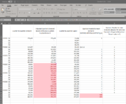
I've got quarterly demand and supply. I need to know how many quarters it will take for the supply to meet each demand

C2 is initial demand (followed by quarterly demand for next in C6) and E2 is initial supply (followed by quarterly supply)

It takes five quarters for the cumulative supply, SUM(E2:E6), to meet the demand,C2

There is leftover demand, SUM(E2:E6-C2), 323,487-276,459=47,028 that needs to be accounted against quarters supply and directly impacts the quarterly drawdown time dynamically column G.

The issue arises when column D becomes negative.

The negative value in represents additional supply that needs to be accounted for in E20 and so forth down column E, a surplus supply gets added to the next quarter's supply.

I used =IFERROR(MATCH(D6,SUBTOTAL(9,OFFSET(OFFSET($E$2,SUM($F$2:F5),0),,,ROW(E6:$E$633)-ROW(E6))),1),1) to calculate the drawdown time required in column F and adjusted each each drawdown time for the previous quarter's required drawdown time, column G.

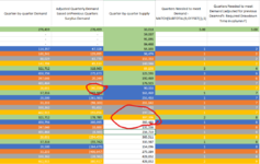
For reference, I color coded how the above formula works.

 

[CA_Punit]

Hi,,

If going through the details i have drawn a sample data using my own helper columns.
If this is what you are looking for than it could be done without helper too.

Book1
	A	B	C	D	E	F	G	H	I	J	K	L
1								Helper Column			Cummulative Quarter	Quarter
2				Cumulative Demand	Supply	Cumulative Supply		If Equals	Condition 3		0
3	FY2021	Q1	276459	276459	33018	33018		0	5		5	5
4		Q2	0	276459	59007	92025		0	5		5	0
5		Q3	0	276459	91891	183916		0	5		5	0
6		Q4	0	276459	55103	239019		0	5		5	0
7	FY2122	Q1	114357	390816	98474	337493		0	6		6	1
8		Q2	160241	551057	153353	490846		0	7		7	1
9		Q3	88029	639086	148240	639086	0	7	8		7	0
10		Q4	142706	781792	69158	708244		0	9		9	2
11	FY2223	Q1	321712	1103504	123593	831837		0	0		0	0
12		Q2	450794	1554298		831837		0	0		0	0
13		Q3	247646	1801944		831837		0	0		0	0
14		Q4		1801944		831837		0	0		0	0
15	FY2324	Q1		1801944		831837		0	0		0	0
16		Q2		1801944		831837		0	0		0	0
17		Q3		1801944		831837		0	0		0	0
18		Q4		1801944		831837		0	0		0	0
19
20
Sheet1

Cell Formulas
Range	Formula
H3:H18	H3	=MAX(IF(IF(D3=$F$3:$F$18,1,0)=1,ROW($F$3:$F$18)-ROW($F$3)+1,0))
I3:I18	I3	=IFERROR(AGGREGATE(15,6,1/(1/(IF(D3<$F$3:$F$18,1,0)*(ROW($F$3:$F$18)-ROW($F$3)+1))),1),0)
K3:K18	K3	=IF(H3>0,H3,I3)
L3:L18	L3	=IF(K3-K2<0,0,K3-K2)
E9	E9	=140966+7274
G9	G9	=D9-F9
D3:D18	D3	=SUM($C$3:C3)
F3:F18	F3	=SUM($E$3:E3)

 

[jjohns829]

Hi,,

If going through the details i have drawn a sample data using my own helper columns.
If this is what you are looking for than it could be done without helper too.

Book1
	A	B	C	D	E	F	G	H	I	J	K	L
1								Helper Column			Cummulative Quarter	Quarter
2				Cumulative Demand	Supply	Cumulative Supply		If Equals	Condition 3		0
3	FY2021	Q1	276459	276459	33018	33018		0	5		5	5
4		Q2	0	276459	59007	92025		0	5		5	0
5		Q3	0	276459	91891	183916		0	5		5	0
6		Q4	0	276459	55103	239019		0	5		5	0
7	FY2122	Q1	114357	390816	98474	337493		0	6		6	1
8		Q2	160241	551057	153353	490846		0	7		7	1
9		Q3	88029	639086	148240	639086	0	7	8		7	0
10		Q4	142706	781792	69158	708244		0	9		9	2
11	FY2223	Q1	321712	1103504	123593	831837		0	0		0	0
12		Q2	450794	1554298		831837		0	0		0	0
13		Q3	247646	1801944		831837		0	0		0	0
14		Q4		1801944		831837		0	0		0	0
15	FY2324	Q1		1801944		831837		0	0		0	0
16		Q2		1801944		831837		0	0		0	0
17		Q3		1801944		831837		0	0		0	0
18		Q4		1801944		831837		0	0		0	0
19
20
Sheet1

Cell Formulas
Range	Formula
H3:H18	H3	=MAX(IF(IF(D3=$F$3:$F$18,1,0)=1,ROW($F$3:$F$18)-ROW($F$3)+1,0))
I3:I18	I3	=IFERROR(AGGREGATE(15,6,1/(1/(IF(D3<$F$3:$F$18,1,0)*(ROW($F$3:$F$18)-ROW($F$3)+1))),1),0)
K3:K18	K3	=IF(H3>0,H3,I3)
L3:L18	L3	=IF(K3-K2<0,0,K3-K2)
E9	E9	=140966+7274
G9	G9	=D9-F9
D3:D18	D3	=SUM($C$3:C3)
F3:F18	F3	=SUM($E$3:E3)

Hi CA_Punit,

This looks good, and I think it'll accomplish my goa, thanks! I do have a question, though, I'm not sure I get the formulas in E9 and G9. Will those have to be manually inseryaed as my raw data increases in scope?

Best,
Matt