Hi Excel experts,
I'm working on a scheduling system for my work and I'm a bit stuck in terms of working out a logical formula that takes the following criteria into consideration and produces an amended figure based on the met criteria.
The decission tree would be as following :
I've achieved this in the formula however I don't know where I'm going wrong for the formula to also apply rules 2-4 and work with the correct figure as at the moment it will not take into consideration which order is higher and/or if there is an order in the revised column.
I know this is chaotically explained but i'm at a point where I've been trying to figure this for hours and i'm myself am confused with all this!
Code from my formula that lives in column L
I'm working on a scheduling system for my work and I'm a bit stuck in terms of working out a logical formula that takes the following criteria into consideration and produces an amended figure based on the met criteria.
The decission tree would be as following :
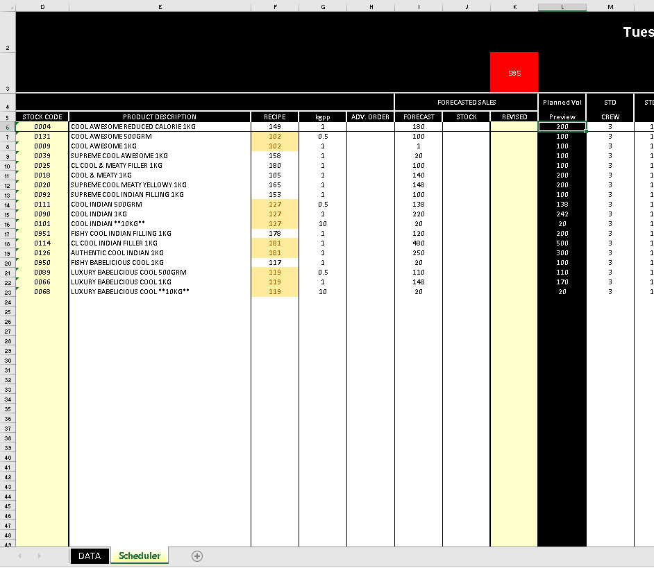
- is there data other than 0 in column D (of each row) if true then proceed otherwise blank
- Is there an order in column I (FORECAST) if so consider this data to be used however,
- if there is an order in column H (ADV. ORDER) then is it higher than data in column I? if it is then use the data in column H instead of column I
- Then look at if there is data in column K (REVISED) and if true then consider data in column K as data to equation over data in columns I & H UNLESS data in column H is higher than in column K
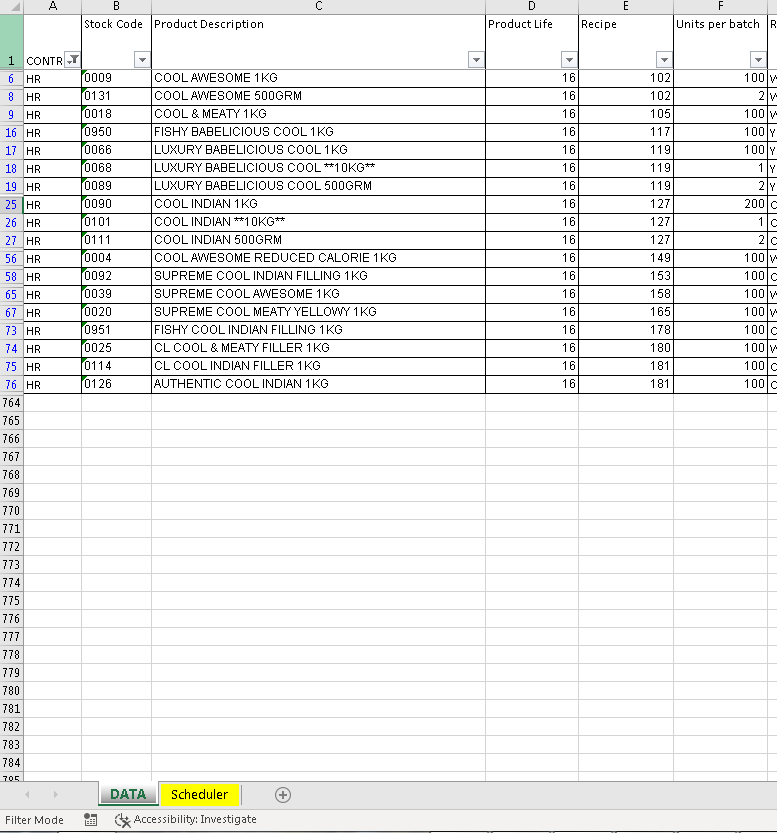
- Now that we have established which orders excel should be taking into consideration we need to do the calculation, but before the calculation it must do another logical equation meaning if data determined in steps 2-4 minus figure in column J is less or equal to 0 then column L to display 0 OTHERWISE it must take the determined order minus data in column J (STOCK) and divide it by batch size, round the result up and multiply again by the batch size (which lives in DATA tab), this will batch the Planned volume up (I've gotten this far on my own and this is where it gets complicated)
- I need to take the take the total of all products with the same recipes (column F) and excel take that total and take away anything that is 0.5 or 10 in column G and take it off the product that is 1 in column G which will leave it with the remainder. The idea is that the total from all products i.e rows 14-16 is a total of a batched up volume in this case (400kg)
I've achieved this in the formula however I don't know where I'm going wrong for the formula to also apply rules 2-4 and work with the correct figure as at the moment it will not take into consideration which order is higher and/or if there is an order in the revised column.
I know this is chaotically explained but i'm at a point where I've been trying to figure this for hours and i'm myself am confused with all this!
Code from my formula that lives in column L
Code:
=IF(COUNTIFS(F:F,F6,G:G,1)>1,IFERROR(IF(IF(K6>0,ROUNDUP((K6-J6)/INDEX(DATA!$B:$H,MATCH(D6,DATA!$B:$B,0),MATCH("Units per batch",DATA!$1:$1,0)-1),0)*INDEX(DATA!$B:$H,MATCH(D6,DATA!$B:$B,0),MATCH("Units per batch",DATA!$1:$1,0)-1),ROUNDUP((MAX(H6,I6)-J6)/INDEX(DATA!$B:$H,MATCH(D6,DATA!$B:$B,0),MATCH("Units per batch",DATA!$1:$1,0)-1),0)*INDEX(DATA!$B:$H,MATCH(D6,DATA!$B:$B,0),MATCH("Units per batch",DATA!$1:$1,0)-1))<0,0,IF(K6>0,ROUNDUP((K6-J6)/INDEX(DATA!$B:$H,MATCH(D6,DATA!$B:$B,0),MATCH("Units per batch",DATA!$1:$1,0)-1),0)*INDEX(DATA!$B:$H,MATCH(D6,DATA!$B:$B,0),MATCH("Units per batch",DATA!$1:$1,0)-1),ROUNDUP((MAX(H6,I6)-J6)/INDEX(DATA!$B:$H,MATCH(D6,DATA!$B:$B,0),MATCH("Units per batch",DATA!$1:$1,0)-1),0)*INDEX(DATA!$B:$H,MATCH(D6,DATA!$B:$B,0),MATCH("Units per batch",DATA!$1:$1,0)-1))),""),
IF(G6=1,IF(K6>0,ROUNDUP(K6/INDEX(DATA!$B:$H,MATCH(D6,DATA!$B:$B,0),MATCH("Units per batch",DATA!$1:$1,0)-1),0)*INDEX(DATA!$B:$H,MATCH(D6,DATA!$B:$B,0),MATCH("Units per batch",DATA!$1:$1,0)-1)-SUMIFS(I:I,F:F,F6,G:G,0.5)-SUMIFS(I:I,F:F,F6,G:G,10),
ROUNDUP(SUMIF(F:F,F6,I:I)/INDEX(DATA!$B:$H,MATCH(D6,DATA!$B:$B,0),MATCH("Units per batch",DATA!$1:$1,0)-1),0)*INDEX(DATA!$B:$H,MATCH(D6,DATA!$B:$B,0),MATCH("Units per batch",DATA!$1:$1,0)-1)-SUMIFS(I:I,F:F,F6,G:G,0.5)-SUMIFS(I:I,F:F,F6,G:G,10)),
IFERROR(IF(IF(K6>0,ROUNDUP((K6-J6)/INDEX(DATA!$B:$H,MATCH(D6,DATA!$B:$B,0),MATCH("Units per batch",DATA!$1:$1,0)-1),0)*INDEX(DATA!$B:$H,MATCH(D6,DATA!$B:$B,0),MATCH("Units per batch",DATA!$1:$1,0)-1),ROUNDUP((MAX(H6,I6)-J6)/INDEX(DATA!$B:$H,MATCH(D6,DATA!$B:$B,0),MATCH("Units per batch",DATA!$1:$1,0)-1),0)*INDEX(DATA!$B:$H,MATCH(D6,DATA!$B:$B,0),MATCH("Units per batch",DATA!$1:$1,0)-1))<0,0,IF(K6>0,ROUNDUP((K6-J6)/INDEX(DATA!$B:$H,MATCH(D6,DATA!$B:$B,0),MATCH("Units per batch",DATA!$1:$1,0)-1),0)*INDEX(DATA!$B:$H,MATCH(D6,DATA!$B:$B,0),MATCH("Units per batch",DATA!$1:$1,0)-1),ROUNDUP((MAX(H6,I6)-J6)/INDEX(DATA!$B:$H,MATCH(D6,DATA!$B:$B,0),MATCH("Units per batch",DATA!$1:$1,0)-1),0)*INDEX(DATA!$B:$H,MATCH(D6,DATA!$B:$B,0),MATCH("Units per batch",DATA!$1:$1,0)-1))),"")))
Last edited by a moderator: