Subtotals Filter when Table is Filtered

[scott11]

Hello,

I have two tables in my spreadsheet. Table 1 allows me to input different orders, companies, and totals. Table 2, looks for key words under Order Type and adds up all the totals that match that key word (as shown in the below example). However, when I filter Table one to include only the totals for Company A, I want the totals in Table 2 to reflect only those totals and not the totals from everything in Table 1. Currently, if I filter out Company B from Table 1 I still show a total of $55 in Table 2, though the new total should equal $40.

My formula for Materials in Table 2 is as follows: =SUMIF($H$13:$H$32,"Materials",$V$13:$V$32), with column H being Order Type and column V being Subtotal.

I can add a final row to the bottom of Table 1 and input a SUM function that will return a sum of only those numbers shown during a filter, but I'm hoping I can show that in Table 2 instead. I've include what it would look like in the second set of pictures below.

Table 1

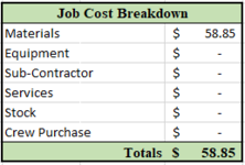
Table 2

 

[Fluff]

How about

=SUMPRODUCT(($H$13:$H$32="Materials")*(SUBTOTAL(3,OFFSET($H$13:$H$32,ROW($H$13:$H$32)-MIN(ROW($H$13:$H$32)),,1))),$V$13:$V$32)

 

[scott11]

If table 1 is a structured table, the simplest way would be to add a total row & link to that.
Otherwise you would need something like

=SUMPRODUCT(($H$13:$H$32="Materials")*(SUBTOTAL(3,OFFSET($H$13:$H$32,ROW($H$13:$H$32)-MIN(ROW($H$13:$H$32)),,1))),$V$13:$V$32)

Thanks Fluff, I'm heading out for the holiday so I will have to look at what you provided on Monday. Happy New Years!

 

[Fluff]

Ok, Happy new year to you. ?

 

[scott11]

Ok, Happy new year to you. ?

That did the trick! Thanks Fluff!

 

[Fluff]

You're welcome & thanks for the feedback.