Sum a range based on another column with dates where the MONTH matches a drop down list in another cell?

NamssoB

Board Regular
Joined
Jul 8, 2005
Messages
76
Office Version
  1. 365
  2. 2016
Platform
  1. Windows
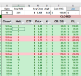
I have a list of stock trades, all dated in column O (from O5:O5000). I have a profit/loss in column U starting at U5. I have a drop down in U1 to select Month (3-letter abbreviation), as well as the word "Total". My goal is to be able to select Jan from the drop down, and have it show me my profit from January. Change to Feb, and I only see profit from Feb. Change to Total, and it shows me total profit.

I want to select Jan, Feb, Mar, etc., in the drop down, and have cell U2 show me a total for all items with a date within the month selected in the drop down. For example:

U1: Drop down, with a list (Total, Jan, Feb, Mar, ...)
U2: Formula I'm trying to figure out: SUM U5:U5000 for any entries with a date (Column O5:O5000, 12-Feb, 5-Jan, etc) that matches the month selected in U1
U5... Values I want to sum
O5... Dates

I know I can use TEXT(O5,"mmm") to grab the 3-letter month and compare it to U1, but I can't figure out how to get that into my formula in U2.

And when I select Total in U2, I just want to add everything up, the entire column U starting at U5.

Ideas?
 

Attachments

  • Capture.PNG
    Capture.PNG
    27.4 KB · Views: 66

Excel Facts

Fastest way to copy a worksheet?
Hold down the Ctrl key while dragging tab for Sheet1 to the right. Excel will make a copy of the worksheet.
Hey,

When you write months such as "Jan", "Feb", "Mar" etc you can access them as a value if you use =MONTH("1/"&$U$1) (where $U$1 is the month in this example, so if it takes "Feb" as the value this formula will return 2) - this can then be compared to the month of the dates in cell O and used as criteria for your formula.

Because you also have to consider the word "Total" you will want to nest this into an IF condition, and check for this word first as it won't like =MONTH("1/"&"Total") of course.

If cell U1 is empty it will return an error, which you could nest an IFERROR into, or give yourself a prompt that cell U1 should be populated, personal preference I suppose!

Try this in cell U2:

IF($U$1="Total",SUM(U5:U5000),SUMPRODUCT((MONTH("1/"&$U$1)=MONTH(O5:O5000))*(U5:U5000)))
 
Upvote 0
Thanks, but with that formula, I get #Value! for anything other than Total in U1.

I tried modifying it to this, and for #SPILL! error:
IF($U$1="Total",SUM(U5:U5000),IF(MONTH("1/"&$U$1)=MONTH(O5:O5000), SUM(U5:U5000),))
 
Upvote 0
Try this. BTW, I suggest that you update your Account details (click your user name at the top right of the forum) so helpers always know what Excel version(s) & platform(s) you are using as the best solution often varies by version. (Don’t forget to scroll down & ‘Save’)

NamssoB.xlsm
OPQRSTU
1Aug
2173.00
3
4
514-Dec13.00
602-Nov109.00
721-Oct(40.00)
820-Oct(38.00)
918-Oct45.00
1006-Sep(41.00)
1123-Aug(32.00)
1222-Aug121.00
1302-Aug84.00
1420-Jul130.00
1520-Jul4.00
1618-Jul32.00
1714-Jul117.00
1827-Jun(7.00)
1923-Jun(44.00)
2017-Jun73.00
2106-Jun46.00
2224-May103.00
2317-May0.00
2414-May58.00
2507-May4.00
2625-Apr(10.00)
2715-Apr10.00
2814-Apr(26.00)
2927-Mar82.00
3016-Mar(57.00)
3101-Mar107.00
3222-Feb(42.00)
3316-Feb37.00
3416-Feb124.00
3514-Feb(47.00)
3612-Feb103.00
3703-Feb(6.00)
3826-Jan117.00
3923-Jan53.00
4013-Jan3.00
Sheet1
Cell Formulas
RangeFormula
U2U2=SUM(FILTER(U5:U5000,IF(U1="Total",O5:O5000>0,TEXT(O5:O5000,"mmm")=U1),0))
 
Upvote 0
Solved! Your formula worked perfectly, thank you! And I also changed my profile, thanks for the tip!

The good news is that I can now take this and apply it to other columns (total # of trades, average trade size, gain/loss per trade, etc.) I'll also modify the ranges to use OFFSET because I use macros/VBA buttons to add new rows. THANK YOU!
 
Upvote 0
Final formula I used, including the offsets:

=SUM(FILTER(OFFSET(U2,3,0):OFFSET(U2,3000,0),IF(U1="Total",OFFSET(O2,3,0):OFFSET(O2,3000,0)>0,TEXT(OFFSET(O2,3,0):OFFSET(O2,3000,0),"mmm")=U1),0))
 
Upvote 0
Ok - new problem with this that I just discovered VERY STRANGE!

- The Worksheet is sorted descending by close date (column O). So blank / unclosed positions are at the top, Feb is next, Jan below that, etc. Once we hit march, then it will be
Blank / Unclosed
Mar
Feb
Jan

If I select Total, it works (it only sums closed positions)
If I select Feb, it works (it only sums Feb positions)
If I select Jan, it FAILS. It sums Jan + the blank/Unclosed positions at the top!

I added some March positions to see if it's "positional", and it appears to NOT be positional and occurs with JAN only. In other words, when I add Mar dates, I get the following:

Total - sums total only
Mar - sums Mar only
Feb - sums Feb only
Jan - sums Jan + BLANKS at top

Then I thought it must be because Jan is at the bottom, so I resorted so Jan is at the top....SAME PROBLEM! For some reason, it's including values entered into any blank unclosed position with the Jan SUM.

Here's the formula I'm using currently.
=SUM(FILTER(OFFSET(U2,3,0):OFFSET(U2,3000,0),IF(U1="Total",OFFSET(O2,3,0):OFFSET(O2,3000,0)>0,TEXT(OFFSET(O2,3,0):OFFSET(O2,3000,0),"mmm")=U1),0))

Even with your original formula without the Offsets, it behaves the same:
=SUM(FILTER(U5:U5000,IF(U1="Total",O5:O5000>0,TEXT(O5:O5000,"mmm")=U1),0))

Disclaimer: For this exact use case, this error isn't a problem because Blank/Unclosed positions will always be $0, hence the sum won't be affected. However, I discovered this error when trying to re-use this formula in other columns that actually have values in the blank fields, and found that they're skewing the data

Some photos to see what it's doing:

$809.52 is correct for JAN, shown below.
1613227984278.png


See how adding $1000 to an unclosed positions gets added to JAN numbers:
1613228050333.png


Correct Total:
1613228154264.png


Total still correct with value in blank position:
1613228193241.png


The same occurs with Mar and Feb. The error seems to occur only with Jan dates.
 
Upvote 0
Solved! Your formula worked perfectly,
Since more than one person suggested a formula, it is a good idea to ensure readers know who you are referring to (eg by quoting a small part like I have above). ;)


I'll also modify the ranges to use OFFSET because I use macros/VBA
Since OFFSET is a volatile function I would avoid that if possible, & it is possible in this case - see my suggestion below.


If I select Jan, it FAILS. It sums Jan + the blank/Unclosed positions at the top!
I think that I have corrected that below.

Try this in U2 instead.

Excel Formula:
=SUM(FILTER(U5:INDEX(U:U,5000),IF(U1="Total",O5:INDEX(O:O,5000)<>"",(TEXT(O5:INDEX(O:O,5000),"mmm")=U1)*(O5:INDEX(O:O,5000)<>"")),0))
 
Upvote 0
Since more than one person suggested a formula, it is a good idea to ensure readers know who you are referring to (eg by quoting a small part like I have above). ;)

Since OFFSET is a volatile function I would avoid that if possible, & it is possible in this case - see my suggestion below.

I think that I have corrected that below.

Try this in U2 instead.

Excel Formula:
=SUM(FILTER(U5:INDEX(U:U,5000),IF(U1="Total",O5:INDEX(O:O,5000)<>"",(TEXT(O5:INDEX(O:O,5000),"mmm")=U1)*(O5:INDEX(O:O,5000)<>"")),0))

Awesome, this worked better - thank you!

The reason I was using OFFSET is because I use a button to add a new record to the top, so formulas in the top row that started out as U5:U5000 change to U6:U5001. Using OFFSET eliminates this. Your new formula about solves the blank record problem perfectly, but not the offset issue. I can easily address this in my VBA code by pasting your formula back into the Cell.Value property when I click on my Add new Record button, but...is there a way to prevent the offset problem without needing to do this, while still enjoying the benefit of your latest formula?
 
Upvote 0
The reason I was using OFFSET is because I use a button to add a new record to the top, so formulas in the top row that started out as U5:U5000 change to U6:U5001. .....Your new formula about solves the blank record problem perfectly, but not the offset issue.
Just change all the references to row 5 in my formula to row 4 and you still shouldn't need OFFSET.

=SUM(FILTER(U4:INDEX(U:U,5000),IF(U1="Total",O4:INDEX(O:O,5000)<>"",(TEXT(O4:INDEX(O:O,5000),"mmm")=U1)*(O4:INDEX(O:O,5000)<>"")),0))
 
Upvote 0
Solution

Forum statistics

Threads
1,214,522
Messages
6,120,019
Members
448,938
Latest member
Aaliya13

We've detected that you are using an adblocker.

We have a great community of people providing Excel help here, but the hosting costs are enormous. You can help keep this site running by allowing ads on MrExcel.com.
Allow Ads at MrExcel

Which adblocker are you using?

Disable AdBlock

Follow these easy steps to disable AdBlock

1)Click on the icon in the browser’s toolbar.
2)Click on the icon in the browser’s toolbar.
2)Click on the "Pause on this site" option.
Go back

Disable AdBlock Plus

Follow these easy steps to disable AdBlock Plus

1)Click on the icon in the browser’s toolbar.
2)Click on the toggle to disable it for "mrexcel.com".
Go back

Disable uBlock Origin

Follow these easy steps to disable uBlock Origin

1)Click on the icon in the browser’s toolbar.
2)Click on the "Power" button.
3)Click on the "Refresh" button.
Go back

Disable uBlock

Follow these easy steps to disable uBlock

1)Click on the icon in the browser’s toolbar.
2)Click on the "Power" button.
3)Click on the "Refresh" button.
Go back
Back
Top