Sum a row with cells that may be blank, and some rows that have letters and numbers.

[rowrow780]

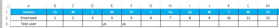
I am creating a vacation and sick tracker. Vacation identified by V. The number of hours will be after the letter V. .
I have tried a formula that has worked when there is no blanks however I have an error when there is blanks. There are blanks as we are only entering Vac hours on the cells ( represents the calendar days ) an employee takes the time.
How would I do this formula to sum total V hours?
Thank you!

 

[Eric W]

Try:

Book1
	A	B	C	D	E	F	G	H	I	J	K	L	M	N	O
1	January	Su	M	T	W	Th	F	Sa	Su	M	T	W	Th	F	Sa
2	Employee	1	2	3	4	5	6	7	8	9	10	11	12
3	Test User				V5	v5				v2
4
5	Sum of vacation
6	12
Sheet3

Cell Formulas
Range	Formula
A6	A6	=SUM(IF(LEFT(B3:M3)="v",MID(B3:M3,2,5)+0))

 

[rowrow780]

Eric, you just saved me hours! Thank you so very much!!!!

 

[Eric W]

Happy to help! Thanks for the update.

 

[rowrow780]

Happy to help! Thanks for the update.

Hi Eric, i've run into a scenerio..
what formula would i use to sum the total hours if an employee will take a combination of sick and vac hours?. Example : v5 ( vacation ) and s3 (sick ) in one day .

TIA!

 

[Sufiyan97]

Try until Eric enters, not too good but works

Book7
	A	B	C	D	E	F	G	H	I	J	K	L	M	N	O
1	January	Su	M	T	W	Th	F	Sa	Su	M	T	W	Th	F	Sa
2	Employee	1	2	3	4	5	6	7	8	9	10	11	12
3	Test User				V5	v5 s3				v2
4
5	Sum of vacation
6	15
7
8
Sheet2

Cell Formulas
Range	Formula
A6	A6	=SUM(IFERROR(LEFT(SUBSTITUTE(SUBSTITUTE(SUBSTITUTE(SUBSTITUTE(B3:M3,"v",0),"V",0),"S",0),"s",0),SEARCH(" ",B3:M3&" ")-1)+0,0))+SUM(IFERROR(MID(SUBSTITUTE(SUBSTITUTE(SUBSTITUTE(SUBSTITUTE(B3:M3,"v",0),"V",0),"S",0),"s",0),SEARCH(" ",B3:M3),5)+0,0))

 

[Eric W]

Thanks Sufiyan97 for stepping in, I kind of lost track of this one. Here's another option:

Book1
	A	B	C	D	E	F	G	H	I	J	K	L	M	N	O
1	January	Su	M	T	W	Th	F	Sa	Su	M	T	W	Th	F	Sa
2	Employee	1	2	3	4	5	6	7	8	9	10	11	12
3	Test User				V5	v5 s3		s1 v4		v2
4
5	Sum of vacation
6	20
7
8	Vacation	16
9	Sick	4
10	Total	20
Sheet2

Cell Formulas
Range	Formula
A6	A6	=SUM(IFERROR(LEFT(SUBSTITUTE(SUBSTITUTE(SUBSTITUTE(SUBSTITUTE(B3:M3,"v",0),"V",0),"S",0),"s",0),SEARCH(" ",B3:M3&" ")-1)+0,0))+SUM(IFERROR(MID(SUBSTITUTE(SUBSTITUTE(SUBSTITUTE(SUBSTITUTE(B3:M3,"v",0),"V",0),"S",0),"s",0),SEARCH(" ",B3:M3),5)+0,0))
B8	B8	=SUM(MID(B3:O3&"v0",SEARCH("v",B3:O3&"v")+1,1)+0)
B9	B9	=SUM(MID(B3:O3&"s0",SEARCH("s",B3:O3&"s")+1,1)+0)
B10	B10	=SUM(B8:B9)

This assumes that the number of hours is always 1 digit. If you want, you can combine the B8 and B9 formulas into one cell easy enough.

 

[rowrow780]

Thank you Eric and Sufiyan! appreciate this!