Sum Column Than Look For Cell

[JMata806]

Greetings I am a green horn in Excel and studying up to make my life fun and efficient.
I've used this site many times to get broaden my knowledge on Excel and thank each and every brain head here!

However, I've hit a dead end and perhaps I am overthinking or just not using the right wording when searching this vast forum.
I am attempting to setup either a VBA or formula to sum off a specific table say (Table 1 is Apples, Table 2 is Oranges, etc) using SUMIFS which helps me get the totals no issues.

Now the roadblock.

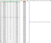
Now I want to know based on this list when said amount reaches a total, say ">=10" upon which it will report a corresponding column that has the date.
So in short it would pull the date of when the sum of a count reaches 10 or more.

In case my words are confusing I drew up a basic idea to help understand my process.

So if you can help me I would greatly appreciate it, I was thinking of using Lookup or such to resolve this but again I've lost myself in trying to resolve this and for all I know it may be simple and I just am looking at this more difficultly than it should.

^_^

 

[jasonb75]

Doing it with a single formula in the output table would need a convoluted combination of sumproduct, offset, subtotal, and others.

Much easier would be a helper column in the source table. Use this In D2, then fill down to create a running total for each item

=SUMIFS(C$2:C2,B$2:B2,B2)

Then you could use MINIFS to extract the date from column A with

=MINIFS($A$2:$A$25,$B$2:$B$25,"Apple",$D$2:$D$25,">=10")

substituting "Apple" in the formula for the cell in the result table that contains the relevant description.

 

[JMata806]

See I was looking at it harder than I should of lol I'll try this out and get back with you but just knowing its using the MINIFS is enough to know it'll work and make it easier.

 

[Eric W]

It's not terrible without a helper column:

Book1
	A	B	C	D	E	F	G
1	Date	Name	Total		Name	Date	Limit
2	1/1/2021	Apple	1		Apple	1/1/2021	10
3	1/1/2021	Banana	2		Banana	1/15/2021
4	1/15/2021	Orange	5		Orange	4/26/2021
5	3/5/2021	Grapes	1		Grapes	N/A
6	4/26/2021	Olives	5		Olives	8/13/2021
7	8/13/2021	Carrots	3		Carrots	N/A
8	2/10/2021	Lettuce	7		Lettuce	11/1/2021
9	1/6/2021	Pumpkins	5		Pumpkins	N/A
10	1/1/2021	Apple	9
11	1/15/2021	Banana	8
12	3/5/2021	Orange	2
13	4/26/2021	Grapes	5
14	8/13/2021	Olives	7
15	12/10/2021	Carrots	0
16	10/3/2021	Lettuce	2
17	1/1/2021	Pumpkins	3
18	1/15/2021	Apple	4
19	3/5/2021	Banana	2
20	4/26/2021	Orange	9
21	8/13/2021	Grapes	1
22	12/10/2021	Olives	6
23	1/1/2022	Carrots	4
24	11/1/2021	Lettuce	2
25	1/15/2021	Pumpkins	1
Sheet2

Cell Formulas
Range	Formula
E2:E9	E2	=UNIQUE(B2:B25)
F2:F9	F2	=IFERROR(SMALL(IF(SUMIFS(C$2:C$25,A$2:A$25,"<="&A$2:A$25,B$2:B$25,E2)>=G$2,$A$2:$A$25),1),"N/A")
Dynamic array formulas.

Depending on your version of Excel, you might not have the UNIQUE function. And you might need to confirm F2 with Control+Shift+Enter.

 

[JMata806]

Let me try with a different example than, cause I think I have it nearly working with MINIFS but see if I am on the right track.
I'll test it with the Unique and IFERRORS here as well just in case, but maybe this will help explain my thought process.

Basically I and summing points =SUMPRODUCT(SUMIFS(B2:B41,C2:C41,E2:E41)), this will give me a total for only the codes that match this list.
But next I want to know based of this list where the 10th or greater point occurred than report back the Date (A) from the corresponding cell.

There are several Category lists I use but figured if I can calculate the first list than I can just transition this to the others.

You guys are amazing on that too thanks so much!

 

[JMata806]

Tried this with my latest concept from above and seem to have trouble where using the

=UNIQUE(C2:C41)
=IFERROR(SMALL(IF(SUMIFS(B$2:B$41,A$2:A$41,"<="&A$2:A$41,C$2:C$41,E2:E41)>=G$2,$A$2:$A$41),1),"N/A")

Where G2 is 10

Seems like its not wanting to use the list from E2:E41 but just unique values only.

Similar here when I attempt trying to make a helper table its refusing to accept comparing the sum points of the table E2:E41 with C2:C41 till it gets to point 10 than giving date from A2:A41.

May be pushing the limits on this though I've tried using =Filter as well, but its limited to 365 I believe and I need to warrant it to compare the sums first.

Still thanks though for the ideas its really helping! Going to try the mini-sheet soon once I am home and have more free time to play with this.

 

[JMata806]

Sadly after a bit neither option worked going to try going back to the beginning and rethink my method.

Though I do want to say thanks the initial idea worked but adding the other variable threw me for a loop lol.