Sum if same ID and same date - only once

[Mariella]

Hi there,

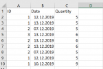
I am trying to sum quantities in a database. Thereby it is important that for each ID, when the date is the same, the value is only added once. I am absolutely struggling to calculate that.

Maybe someone can help me? I would really appreciate it!

Best,
Mariella

 

[sandy666]

like this?

you can do that with Power Query (Get&Transform)

// Table1
let
    Source = Excel.CurrentWorkbook(){[Name="Table1"]}[Content],
    Type = Table.TransformColumnTypes(Source,{{"Date", type date}}),
    Group = Table.Group(Type, {"ID", "Date"}, {{"Qty", each List.Sum([Quantity]), type number}}),
    Sort = Table.Sort(Group,{{"ID", Order.Ascending}, {"Date", Order.Ascending}})
in
    Sort

 

[jasonb75]

There are probably many ways that you could do this, the first one that comes to mind is to add a helper column with adjusted quantities then sum that column.

Try this formula in D2, filled down to D10, then sum column D with a pivot table.

=C2/COUNTIFS($A$2:$A$10,A2,$B$2:$B$10,B2)

Book1
	A	B	C	D	E	F	G
1	id	date	qty	adj qty		ID	Sum of adj qty
2	1	12/12/2019	5	2.5		1	19
3	1	13/12/2019	5	5		2	11
4	2	07/12/2019	5	2.5		3	6
5	3	13/12/2019	6	6		Grand Total	36
6	2	13/12/2019	6	3
7	2	13/12/2019	6	3
8	2	07/12/2019	5	2.5
9	1	12/12/2019	5	2.5
10	1	10/12/2019	9	9
Sheet7

Cell Formulas
Range	Formula
D2:D10	D2	=C2/COUNTIFS($A$2:$A$10,A2,$B$2:$B$10,B2)

 

[sandy666]

or like this

// Table1
let
    Source = Excel.CurrentWorkbook(){[Name="Table1"]}[Content],
    Type = Table.TransformColumnTypes(Source,{{"Date", type date}}),
    Dups = Table.Distinct(Type, {"ID", "Date"}),
    Group = Table.Group(Dups, {"ID", "Date"}, {{"Qty", each List.Sum([Quantity]), type number}}),
    Sort = Table.Sort(Group,{{"ID", Order.Ascending}, {"Date", Order.Ascending}})
in
    Sort

 

[Mariella]

There are probably many ways that you could do this, the first one that comes to mind is to add a helper column with adjusted quantities then sum that column.

Try this formula in D2, filled down to D10, then sum column D with a pivot table.

=C2/COUNTIFS($A$2:$A$10,A2,$B$2:$B$10,B2)

Book1
	A	B	C	D	E	F	G
1	id	date	qty	adj qty		ID	Sum of adj qty
2	1	12/12/2019	5	2.5		1	19
3	1	13/12/2019	5	5		2	11
4	2	07/12/2019	5	2.5		3	6
5	3	13/12/2019	6	6		Grand Total	36
6	2	13/12/2019	6	3
7	2	13/12/2019	6	3
8	2	07/12/2019	5	2.5
9	1	12/12/2019	5	2.5
10	1	10/12/2019	9	9
Sheet7

Cell Formulas
Range	Formula
D2:D10	D2	=C2/COUNTIFS($A$2:$A$10,A2,$B$2:$B$10,B2)

Thanks Jason for the quick answer! This is the right idea and works perfectly for the given dataset. Unfortunately, if I have a third time (or more) the same ID and date it doesn't work anymore...
Do you have an idea how I could adjust this. I don't really understand the formula so it is hard to adapt for me.

Best,
Mariella

 

[Mariella]

or like this
View attachment 3768

// Table1
let
    Source = Excel.CurrentWorkbook(){[Name="Table1"]}[Content],
    Type = Table.TransformColumnTypes(Source,{{"Date", type date}}),
    Dups = Table.Distinct(Type, {"ID", "Date"}),
    Group = Table.Group(Dups, {"ID", "Date"}, {{"Qty", each List.Sum([Quantity]), type number}}),
    Sort = Table.Sort(Group,{{"ID", Order.Ascending}, {"Date", Order.Ascending}})
in
    Sort

Hey
This one looks right. I have absolutely no idea how to use code in Excel but I will try to figure that out!
Thanks you!!
Best,
Mariella

 

[sandy666]

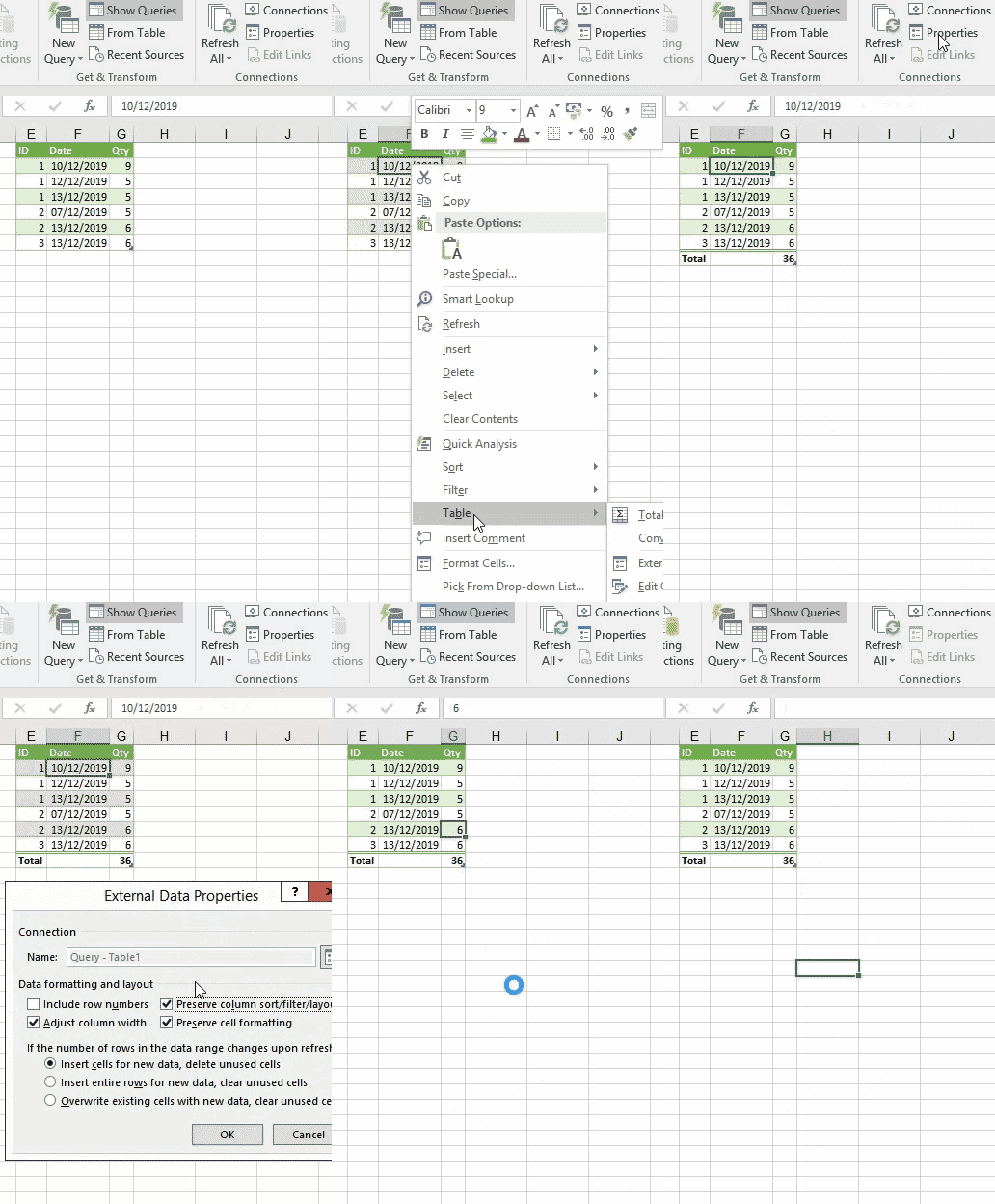
select your original table
from the ribbon Data - From Table
then in Power Query Editor open Advanced Editor
and replace all code there with code copied from the post
then Done , Close&Load

after that:

 

[Mariella]

There are probably many ways that you could do this, the first one that comes to mind is to add a helper column with adjusted quantities then sum that column.

Try this formula in D2, filled down to D10, then sum column D with a pivot table.

=C2/COUNTIFS($A$2:$A$10,A2,$B$2:$B$10,B2)

Book1
	A	B	C	D	E	F	G
1	id	date	qty	adj qty		ID	Sum of adj qty
2	1	12/12/2019	5	2.5		1	19
3	1	13/12/2019	5	5		2	11
4	2	07/12/2019	5	2.5		3	6
5	3	13/12/2019	6	6		Grand Total	36
6	2	13/12/2019	6	3
7	2	13/12/2019	6	3
8	2	07/12/2019	5	2.5
9	1	12/12/2019	5	2.5
10	1	10/12/2019	9	9
Sheet7

Cell Formulas
Range	Formula
D2:D10	D2	=C2/COUNTIFS($A$2:$A$10,A2,$B$2:$B$10,B2)

OMG never mind - it works! It is then dividing by 3. I also understood the formula!

 

[Peter_SSs]

If the same ID and Date always has the same qty like your samples, then without a helper column, you could try this, copied down.

Book1
	A	B	C	D	E	F	G
1	id	date	qty			ID	Sum Once
2	1	12/12/2019	5			1	19
3	1	13/12/2019	5			2	11
4	2	7/12/2019	5			3	6
5	3	13/12/2019	6
6	2	13/12/2019	6
7	2	13/12/2019	6
8	2	7/12/2019	5
9	1	12/12/2019	5
10	1	10/12/2019	9
Sum

Cell Formulas
Range	Formula
G2:G4	G2	=SUMPRODUCT((A$2:A$10=F2)*(MATCH(A$2:A$10&"|"&B$2:B$10,A$2:A$10&"|"&B$2:B$10,0)=ROW(A$2:A$10)-ROW(A$2)+1),C$2:C$10)

 

[Mariella]

If the same ID and Date always has the same qty like your samples, then without a helper column, you could try this, copied down.

Book1
	A	B	C	D	E	F	G
1	id	date	qty			ID	Sum Once
2	1	12/12/2019	5			1	19
3	1	13/12/2019	5			2	11
4	2	7/12/2019	5			3	6
5	3	13/12/2019	6
6	2	13/12/2019	6
7	2	13/12/2019	6
8	2	7/12/2019	5
9	1	12/12/2019	5
10	1	10/12/2019	9
Sum

Cell Formulas
Range	Formula
G2:G4	G2	=SUMPRODUCT((A$2:A$10=F2)*(MATCH(A$2:A$10&"|"&B$2:B$10,A$2:A$10&"|"&B$2:B$10,0)=ROW(A$2:A$10)-ROW(A$2)+1),C$2:C$10)

Hi Peter,
Thank you very much! Indeed, this would work and I thought about this before but my original dataset contains 95000 rows and I would have to list the options before

So nice that Excel even provides different ways to come to a solution! Everything worked out!

Best,
Mariella