Sum Material Based on Different Criteria

[nathanthomson11]

Unfortunately the office restricts my ability to upload a file so I'll do my best to explain what I'm looking for based on the attached image.

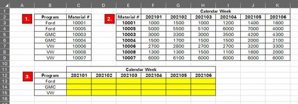
What I am trying to do is sum in table #3 based on information from Table #1 & Table #2. For example, in C13, I want to sum all of "Ford" material in Table #2 under the matching Calendar week - in this case "202101". However, in order to know what material in Table #2 is "Ford", it also needs to reference Table #1 to see what material number belongs to "Ford". The total in C13 should be 6,000 - the sum of "10001" & "10005" under calendar week "202101".

I suspect it's either a SUMPRODUCT or INDEXMATCH but I can't find a proper combination.

 

[mamady]

Hi Dear,

Please check if the below satisfies your requirement:

Book1
	B	C	D	E	F	G	H	I	J	K
2	Program	Material #		Material #	202101	202102	202103	202104	202105	202106
3	Ford	10001		10001	1000	1500	1000	1200	1400	1600
4	Ford	10005		10005	5000	5500	5100	6000	7000	4000
5	GMC	10003		10003	3000	3300	3000	3500	4200	4300
6	GMC	10004		10004	1500	1700	1500	1500	2000	2100
7	VW	10006		10006	2700	2800	2700	2700	3200	3300
8	VW	10008		10008	1300	1300	1500	1100	1600	2000
9	VW	10007		10007	6000	6100	6000	6000	6000	6000
10
11
12	Program	202101	202102	202103	202104	202105	202106
13	Ford	6000	7000	6100	7200	8400	5600
14	GMC	4500	5000	4500	5000	6200	6400
15	VW	10000	10200	10200	9800	10800	11300
16		TRUE	TRUE	TRUE	TRUE	TRUE	TRUE
Sheet3

Cell Formulas
Range	Formula
C13:H15	C13	=SUM(SUMIFS(F$3:F$9,$E$3:$E$9,$C$3:$C$9,$B$3:$B$9,$B13))
C16:H16	C16	=SUM(F3:F9)=SUM(C13:C15)

Regards

 

[Peter_SSs]

Please check if the below satisfies your requirement:

That relies on the values in C3:C9 exactly matching the values in E3:E9. I suspect that may not be the case with the OP's actual data else you could just use this.

21 02 10.xlsm
	B	C	D	E	F	G	H	I	J	K
2	Program	Material #		Material #	202101	202102	202103	202104	202105	202106
3	Ford	10001		10001	1000	1500	1000	1200	1400	1600
4	Ford	10005		10005	5000	5500	5100	6000	7000	4000
5	GMC	10003		10003	3000	3300	3000	3500	4200	4300
6	GMC	10004		10004	1500	1700	1500	1500	2000	2100
7	VW	10006		10006	2700	2800	2700	2700	3200	3300
8	VW	10008		10008	1300	1300	1500	1100	1600	2000
9	VW	10007		10007	6000	6100	6000	6000	6000	6000
10
11
12	Program	202101	202102	202103	202104	202105	202106
13	Ford	6000	7000	6100	7200	8400	5600
14	GMC	4500	5000	4500	5000	6200	6400
15	VW	10000	10200	10200	9800	10800	11300
Test1

Cell Formulas
Range	Formula
C13:H15	C13	=SUMIF($B$3:$B$9,$B13,F$3:F$9)

If the order in table 1 may not be identical to table 2 (below I have swapped the two yellow rows) then try ..

21 02 10.xlsm
	B	C	D	E	F	G	H	I	J	K
2	Program	Material #		Material #	202101	202102	202103	202104	202105	202106
3	Ford	10001		10001	1000	1500	1000	1200	1400	1600
4	VW	10008		10005	5000	5500	5100	6000	7000	4000
5	GMC	10003		10003	3000	3300	3000	3500	4200	4300
6	GMC	10004		10004	1500	1700	1500	1500	2000	2100
7	VW	10006		10006	2700	2800	2700	2700	3200	3300
8	Ford	10005		10008	1300	1300	1500	1100	1600	2000
9	VW	10007		10007	6000	6100	6000	6000	6000	6000
10
11
12	Program	202101	202102	202103	202104	202105	202106
13	Ford	6000	7000	6100	7200	8400	5600
14	GMC	4500	5000	4500	5000	6200	6400
15	VW	10000	10200	10200	9800	10800	11300
Test2

Cell Formulas
Range	Formula
C13:H15	C13	=SUMPRODUCT(--(INDEX($B$3:$B$9,MATCH($E$3:$E$9,$C$3:$C$9,0))=$B13),F$3:F$9)

Further, if the calendar weeks in table 2 do not exactly match the calendar weeks in table 3 (I have also swapped the green values) then you could try this

21 02 10.xlsm
	B	C	D	E	F	G	H	I	J	K
2	Program	Material #		Material #	202101	202102	202103	202104	202105	202106
3	Ford	10001		10001	1000	1500	1000	1200	1400	1600
4	VW	10008		10005	5000	5500	5100	6000	7000	4000
5	GMC	10003		10003	3000	3300	3000	3500	4200	4300
6	GMC	10004		10004	1500	1700	1500	1500	2000	2100
7	VW	10006		10006	2700	2800	2700	2700	3200	3300
8	Ford	10005		10008	1300	1300	1500	1100	1600	2000
9	VW	10007		10007	6000	6100	6000	6000	6000	6000
10
11
12	Program	202101	202104	202103	202102	202105	202106
13	Ford	6000	7200	6100	7000	8400	5600
14	GMC	4500	5000	4500	5000	6200	6400
15	VW	10000	9800	10200	10200	10800	11300
Test3

Cell Formulas
Range	Formula
C13:H15	C13	=SUMPRODUCT(--(INDEX($B$3:$B$9,MATCH($E$3:$E$9,$C$3:$C$9,0))=$B13),INDEX($F$3:$K$9,0,MATCH(C$12,$F$2:$K$2,0)))

 

[Marcelo Branco]

Peter,

Curiously this formula (2nd example) didn't work for me in Excel 2010.
=SUMPRODUCT(--(INDEX($B$3:$B$9,MATCH($E$3:$E$9,$C$3:$C$9,0))=$B13),F$3:F$9)

I've gotten a #VALUE error

I have had to use a more complicated array formula.
=SUMPRODUCT(--(INDEX($B$3:$B$9,N(IF(1,MATCH($E$3:$E$9,$C$3:$C$9,0))))=$B13),F$3:F$9)
confirmed with Ctrl+Shift+Enter

Regards

M.

 

[Marcelo Branco]

Adding to my previous post
Didn't work in Excel 2019 either (another machine i have)

Only the mentioned array formula above worked properly

M.

 

[Peter_SSs]

Hi Marcelo
Thanks for pointing those things out. I have difficulty remembering what works in what versions as I only have Excel 365 now. ?
Hopefully we will find out which one(s) work for the OP with Excel 2019.

 

[nathanthomson11]

Apologies for the lack of response guys - I had to table this project for a while but am back at it!

@Peter_SSs, the formula below seems to be working with one caveat - sometimes the two lists (B3:B9) & (E3:#9) don't have the exact same numbers which in this case , if one is missing, it gives me #N/A error.

Any suggestions to fix this?

Range	Formula
Cell Formulas
C13:H15	C13	=SUMPRODUCT(--(INDEX($B$3:$B$9,MATCH($E$3:$E$9,$C$3:$C$9,0))=$B13),INDEX($F$3:$K$9,0,MATCH(C$12,$F$2:$K$2,0)))

 

[Peter_SSs]

sometimes the two lists (B3:B9) & (E3:#9) don't have the exact same numbers

Did you mean (C3:C9) & (E3:E9)?

Try

21 02 10.xlsm
	B	C	D	E	F	G	H	I	J	K
1
2	Program	Material #		Material #	202101	202102	202103	202104	202105	202106
3	Ford	10001		98765	1000	1500	1000	1200	1400	1600
4	VW	10008		10005	5000	5500	5100	6000	7000	4000
5	GMC	10003		10003	3000	3300	3000	3500	4200	4300
6	GMC	10004		22222	1500	1700	1500	1500	2000	2100
7	VW	10006		10006	2700	2800	2700	2700	3200	3300
8	Ford	10005		10008	1300	1300	1500	1100	1600	2000
9	VW	10007		10007	6000	6100	6000	6000	6000	6000
10
11
12	Program	202101	202104	202103	202102	202105	202106
13	Ford	1300	1100	1500	1300	1600	2000
14	GMC	3000	3500	3000	3300	4200	4300
15	VW	13700	14700	13800	14400	16200	13300
Test4

Cell Formulas
Range	Formula
C13:H15	C13	=SUMPRODUCT($F$3:$K$9*($F$2:$K$2=C$12)*(ISNUMBER(MATCH($E$3:$E$9,$C$3:$C$9,0)))*($B$3:$B$9=$B13))

 

[nathanthomson11]

Thank you for the quick response @Peter_SSs ! I think we are close however this formula doesn't seem to be calculating properly. For example, VW under 202101 should equal 10,000 (F7 + F8 + F9) but it is showing 13,700.

 

[Peter_SSs]

Let's try a change of approach then.

nathanthomson11.xlsm
	B	C	D	E	F	G	H	I	J	K
1
2	Program	Material #		Material #	202101	202102	202103	202104	202105	202106
3	Ford	10001		98765	1000	1500	1000	1200	1400	1600
4	VW	10008		10005	5000	5500	5100	6000	7000	4000
5	GMC	10003		10003	3000	3300	3000	3500	4200	4300
6	GMC	10004		22222	1500	1700	1500	1500	2000	2100
7	VW	10006		10006	2700	2800	2700	2700	3200	3300
8	Ford	10005		10008	1300	1300	1500	1100	1600	2000
9	VW	10007		10007	6000	6100	6000	6000	6000	6000
10
11
12	Program	202101	202104	202103	202102	202105	202106
13	Ford	5000	6000	5100	5500	7000	4000
14	GMC	3000	3500	3000	3300	4200	4300
15	VW	10000	9800	10200	10200	10800	11300
Test5

Cell Formulas
Range	Formula
C13:H15	C13	=SUM(FILTER(FILTER($F$3:$K$9,$F$2:$K$2=C$12),ISNUMBER(MATCH($E$3:$E$9,FILTER($C$3:$C$9,$B$3:$B$9=$B13),0))))