Sum of values based on variable values

[PRADEEPSWALSE]

Hi,
I need help for addition of variable values.
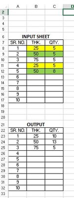
E.g. Values in column 'B' are variable. I want SUM of values mentioned in column 'C' based on values of column 'B'. I have total 10 rows. Values of column 'B' are variable and it will be entered by user. Some cell may be empty. Refer attached Images for easy understanding.

Please suggest solution for this query.
Thanks in advance.

Regards,
Pradeep

 

[jasonb75]

This will do it. Note that I've added an extra column to the Input table, I don't see that it will be possible to do it without that using your version of excel.

I notice that your sample results are sorted in ascending order by size then thk, if the order is not essential then I could possibly shorten the formulas a bit. (not tried it yet).

There are 2 output tables, one for your version of excel and another using office 365 dynamic arrays so that you can compare the difference. Note with the 365 version, the column that I added to the input table is not needed and most of the formulas are much shorter.

Book1 (version 1)19.2.21.xlsx
	A	B	C	D	E	F	G	H	I
4	no	size	thk	qty	Rank
5	1	0.75"	25	5	75.96
6	2	1.5"	50	5	150.98
7	3	1.5"	75	5	150.9866667
8	4	0.75"	25	5	75.96
9	5	1.5"	50	8	150.98
10	6	0.75"	25	10	75.96
11	7	0.75"	100	2	75.99
12	8	3"	100	2	300.99
13	9	1.5"	75	10	150.9866667
14	10	0.75"	100	6	75.99
15	11
16	12
17	13
18	14
19	15
20
21
22
23		Excel 2007 - 2019					Office 365
24	no	size	thk	qty		no	size	thk	qty
25	1	0.75"	25	20		1	0.75"	25	20
26	2	0.75"	100	8		2	0.75"	100	8
27	3	1.5"	50	13		3	1.5"	50	13
28	4	1.5"	75	15		4	1.5"	75	15
29	5	3"	100	2		5	3"	100	2
30	6
Sheet11

Cell Formulas
Range	Formula
E5:E19	E5	=IF(OR(B5="",C5=""),"",SUBSTITUTE(B5,"""","")*100+(1-1/C5))
B25:C30	B25	=IFERROR(INDEX(B$5:B$19,MATCH(SMALL($E$5:$E$19,SUMPRODUCT(COUNTIFS($B$5:$B$19,$B$24:$B24,$C$5:$C$19,$C$24:$C24))+1),$E$5:$E$19,0)),"")
D25:D30	D25	=IF(C25="","",SUMIFS($D$5:$D$19,$B$5:$B$19,B25,$C$5:$C$19,C25))
F25:F29	F25	=SEQUENCE(ROWS(G25#))
G25:H29	G25	=SORT(UNIQUE(FILTER(B5:C19,B5:B19<>"","")))
I25:I29	I25	=SUMIFS(D5:D19,B5:B19,INDEX(G25#,,1),C5:C19,INDEX(G25#,,2))
Dynamic array formulas.