Sum of vlookup in multiple rows with condition

[balaba]

Hi,

Let me try and explain what I need with a simplified example:


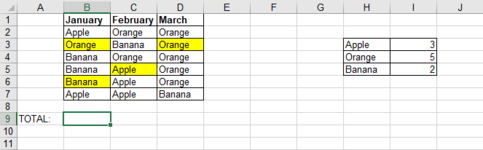
I have a table (H3:I5) that gives me the value for each item (I have dozens of items in the reality).
I need, for each month (in B9, C9, D9), to know the sum of the value of each item for the particular month... but only counting the cells that are NOT in yellow.

For example, for January, it would be:
Apple: 3
Orange: do not count
Banana: 2
Banana: 2
Banana: do not count
Apple: 3
TOTAL=10 -> this is the value that I need

I can't do a formula with vlookup+vlookup+vlookup...

For the color part, I have created a new function (via macro) "colorindex", that gives me the color index of a cell (ex: colorindex(B3) would give me "6" as yellow is color coded as 6 in Excel).

thanks for you help!

 

[Fluff]

Hi & welcome to MrExcel.
Can you post the code for your UDF

 

[MrD31]

Hi,

I don't think there is a formula that allow you to total the column and cells without counting the coloured cells. But I am welcomed to be corrected.

You would need to create a new reference in Formulas > name manager > New.
Then provide a name of the reference and then enter in the scopes to: GET.CELL(38,Sheet1!B2) > hit OK

Then you need to press the equals key against your data(Say your data starts from B2 then press the equals key in C2) and then click to find your named reference and drag it down to the end of the column.

You would need insert a new column against your data for each separate one.

Then you can use the countif function using your reference as the range without including the number 6.

Hopefully this would help if you do not wish to use VBA.

 

[Fluff]

@MrD31
The OP already has a UDF for finding the coloured cells..

 

[balaba]

Hi & welcome to MrExcel.
Can you post the code for your UDF

Hi, thank you!

see below:

Function ColorIndex(CellColor As Range)

ColorIndex = CellColor.Interior.ColorIndex

End Function

 

[Fluff]

Ok, if you change your UDF to

Function ColorIndx(CellColor As Range) As Variant
   Dim Cl As Range
   Dim i As Long
   Dim Ary As Variant
   ReDim Ary(1 To CellColor.Count, 1 To 1)
      For Each Cl In CellColor
         i = i + 1
         Ary(i, 1) = Cl.Interior.ColorIndex
      Next Cl
      ColorIndx = Ary
End Function

you can use it like

+Fluff 1.xlsm
	A	B	C	D	E	F	G	H	I
1		January	February	March
2		Apple	Orange
3		Orange	Banana					Apple	3
4		Banana	Orange					Orange	5
5		Banana	Apple					Banana	2
6		Banana	Apple
7		Apple	Apple
8
9		10	18
10
Master

Cell Formulas
Range	Formula
B9:C9	B9	=SUM(IF(colorIndx(B2:B7)<>6,XLOOKUP(B2:B7,$H$3:$H$5,$I$3:$I$5),0))

 

[balaba]

Amazing, it works perfectly!

Thanks for your help!

 

[Fluff]

You're welcome & thanks for the feedback.