Sum portion of row based on multiple column header criteria

[Bluefish74274]

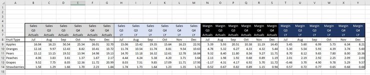
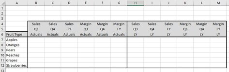
Hi folks! I'm new to the forum so please forgive any newbie faux pas! I've been scouring the web this afternoon (as well as this forum, which I love!) for a solution to my problem. I have monthly metrics (sales, margin, etc.,) for actuals, budget and last year for various fruit. On another tab in my excel spreadsheet, I'd like to be able to aggregate each metric to quarterly or FY totals. So for example, I'd like Q4 Actual sales or Q4 sales margin for last year. Unfortunately sumproduct is not an option as my raw data is 1K columns wide. Also, I realize that I could append subtotals to the raw data which would significantly widen the data and would be very labor intensive. Was hoping this could be done with sumif +index + match, however I tried using '&' to concatenate the multiple match column criteria (Sales + Actuals + Q4), but as you probably already know, the array formula wouldn't work with sumif. I'm hoping there is a solution that doesn't require VBA code, so please bring it on!! Please let me know if you need anything further.

 

[ExcelGzh]

Bluefish74274

Is the image you posted the place where you want these formulas to be or is it the raw data? If it is not the raw data, could you post a sample of that.

 

[jasonb75]

I was wondering the same thing, looking at the screen capture I don't see how that could end up with 1k+ columns of data for just current and previous years but reading the question in detail infers that it is raw data.

@Bluefish74274 does this help with what you're trying to do? (note that this uses random values, not the figures from your example).

gtd562 CountIF.xlsx
	A	B	C	D	E	F	G	H	I	J	K	L	M	N	O	P	Q	R	S	T	U	V	W	X	Y
5		Sales	Sales	Sales	Sales	Sales	Sales	Sales	Sales	Sales	Sales	Sales	Sales	Margin	Margin	Margin	Margin	Margin	Margin	Margin	Margin	Margin	Margin	Margin	Margin
6		Q3	Q3	Q3	Q4	Q4	Q4	Q3	Q3	Q3	Q4	Q4	Q4	Q3	Q3	Q3	Q4	Q4	Q4	Q3	Q3	Q3	Q4	Q4	Q4
7		Actuals	Actuals	Actuals	Actuals	Actuals	Actuals	LY	LY	LY	LY	LY	LY	Actuals	Actuals	Actuals	Actuals	Actuals	Actuals	LY	LY	LY	LY	LY	LY
8	Fruit	Jul	Aug	Sep	Oct	Nov	Dec	Jul	Aug	Sep	Oct	Nov	Dec	Jul	Aug	Sep	Oct	Nov	Dec	Jul	Aug	Sep	Oct	Nov	Dec
9	Apples	2.80	18.81	14.11	4.84	17.84	3.18	3.34	4.23	0.99	3.80	4.73	4.66	3.58	16.22	8.13	9.00	14.96	15.06	12.30	8.18	8.36	5.50	10.53	16.95
10	Oranges	7.02	11.53	9.40	4.95	7.22	9.92	18.55	18.30	13.15	9.48	12.45	17.57	17.28	17.22	16.63	11.86	7.28	15.62	2.71	10.22	19.62	3.56	13.94	16.49
11	Pears	2.44	1.99	13.88	3.66	19.23	4.19	10.62	2.58	18.34	10.34	18.99	0.92	7.85	11.60	12.33	19.73	12.25	4.29	5.86	6.29	4.32	10.89	15.05	17.48
12	Peaches	16.69	11.92	9.53	7.42	17.73	17.65	11.65	5.80	9.77	9.06	8.10	19.79	2.08	9.23	16.67	12.58	0.88	9.23	1.83	17.62	12.78	2.62	5.47	15.97
13	Grapes	6.44	13.64	13.46	2.78	9.97	16.34	6.59	3.82	16.16	2.41	0.96	12.77	17.62	10.19	17.77	12.22	1.30	3.95	16.61	8.27	13.06	13.08	17.14	7.11
14	Strawberries	5.76	9.77	10.07	2.43	19.59	2.72	15.68	12.33	17.68	6.59	9.56	17.85	9.91	3.90	19.38	2.00	7.91	8.25	2.61	17.25	12.79	12.11	5.36	7.05
15
16		Actuals	LY	Actuals	LY
17		Sales	Sales	Margin	Margin
18	Q1	0	0	0	0
19	Q2	0	0	0	0
20	Q3	179.26	189.58	217.59	180.68
21	Q4	171.66	170.03	168.37	196.3
22	Year	350.92	359.61	385.96	376.98
Sheet4

Cell Formulas
Range	Formula
B18:E21	B18	=SUM(FILTER($B$9:$Y$14,($B$5:$Y$5=B$17)*($B$6:$Y$6=$A18)*($B$7:$Y$7=B$16),0))
B22:E22	B22	=SUM(B18:B21)

 

[Bluefish74274]

Yes the data I posted is a small sampling of the raw data. Numerous other metrics are contained in the raw data spreadsheet. Also it was implied but I should have specified that the aggregate totals on different tabs that I am looking for, would be for each fruit, not total of all fruit.

 

[jasonb75]

That should be as simple as reducing the first range of FILTER to a single row and making it relative, although it will most likely need some other minor adjustments to make things work smoothly.

A quick example of how you want the results laid out would give us more to work with.

 

[Bluefish74274]

For simplicity, the format in the attached image will be adequate.

 

[jasonb75]

Something like this (using same raw data as my earlier post)?

gtd562 CountIF (version 1).xlsb
	A	B	C	D	E	F	G	H	I	J	K	L	M
16		Sales	Sales	Sales	Margin	Margin	Margin	Sales	Sales	Sales	Margin	Margin	Margin
17		Q3	Q4	FY	Q3	Q4	FY	Q3	Q4	FY	Q3	Q4	FY
18	Fruit	Actuals	Actuals	Actuals	Actuals	Actuals	Actuals	LY	LY	LY	LY	LY	LY
19	Apples	35.72	25.86	61.58	27.93	39.02	66.95	8.56	13.19	21.75	28.84	32.98	61.82
20	Oranges	27.95	22.09	50.04	51.13	34.76	85.89	50.00	39.50	89.50	32.55	33.99	66.54
21	Pears	18.31	27.08	45.39	31.78	36.27	68.05	31.54	30.25	61.79	16.47	43.42	59.89
22	Peaches	38.14	42.80	80.94	27.98	22.69	50.67	27.22	36.95	64.17	32.23	24.06	56.29
23	Grapes	33.54	29.09	62.63	45.58	17.47	63.05	26.57	16.14	42.71	37.94	37.33	75.27
24	Strawberries	25.60	24.74	50.34	33.19	18.16	51.35	45.69	34.00	79.69	32.65	24.52	57.17
Sheet4

Cell Formulas
Range	Formula
B19:C24,E19:F24,H19:I24,K19:L24	B19	=SUM(XLOOKUP($A19,$A$9:$A$14,FILTER($B$9:$Y$14,($B$5:$Y$5=B$16)*($B$6:$Y$6=B$17)*($B$7:$Y$7=B$18),0)))
D19:D24,G19:G24,J19:J24,M19:M24	D19	=SUM(B19:C19)

 

[Bluefish74274]

Thanks @jasonb75. This formula would work great were if it were not for the fact that I would have to specify the look up range for every metric. Given the fact that the raw data has 1K columns, this would be a heavy lift. The aggregate format I sent was just a sample of metrics that I am looking to summarize. Additional examples include: Promotional sales, non-promotional margin. In addition, not just looking at actuals and last year, also looking for aggregates on budget and forecast. So my goal is to find a more automated formula that won't rely entering each lookup range designation. Hope that makes sense.

 

[Bluefish74274]

I tried out your solution and unfortunately my version of excel doesn't recognize xlookup and filter functions

 

[jasonb75]

If you don't have those functions then I'm guessing that you don't have office 365 as shown on your profile, if you do then it is possibly behind on updates.

I don't think that you're going to be able to automate anything to the point of not setting out the column headings (rows 16 to 18 in the example above), once that is done it is simply a case of entering the first formula (ctrl enter into 2 columns), use Alt + = in the third column for the basic sum then using autofill to populate the rest of the table from those 3 cells.

That said, without the xlookup and filter functions the formula would need to be rewritten using other functions but the setup would be much the same.

The layout of the raw data is not going to work with a pivot table, which only leaves vba or possibly power query, although to be honest I wouldn't know where to start with that.