sum product with conditional start date and end date / end date blank failure

[soychristophe]

Hello Community, I have a block from which I can't get out....

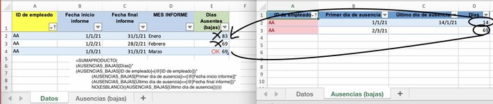
I am using the formula sumaproduct to get the data of the sheet Absences with its first day and its last day, the problem I get when in the last day data there is no date, it is understood or it could be calculated with the formula today() to give you a data. The question is that when there is no date, the summaproduct that I have made adds up the total of days and even in a month that there is no initial or final date.

How can I solve it?

Thank you very much

CONSULTA.xlsx
	A	B	C	D	E
1	ID de empleado	Fecha inicio informe	Fecha final informe	MES INFORME	Dias Ausentes (bajas)
2	AA	1/1/21	1/31/21	Enero	83 [/ FORMULA] [/ XD] [/ XR] [XR] [XH] 3 [/ XH] [XD = h: l | v : t | ch: 24 | cls: bl bt bb ww] AA [/ XD] [XD = cls: bt bb | tx: 44228] 2/1/21 [/ XD] [XD = cls: bt bb | tx: 44255] 2/28/21 [/ XD] [XD = h: l | cls: bt bb] February [/ XD] [XD = fw: b | fz: 18pt | cls: fx bt br bb] [FORMULA == SUMPRODUCT ( (ABSENCES_LOW & lsqb; Days & rsqb;) * (AUSENCIAS_BAJAS[ID de empleado]=[@[ID de empleado]])* (ABSENCES_LAY & lsqb; First day of absence & rsqb;> = & lsqb; @ & lsqb; Report start date & rsqb; & rsqb; * (ABSENCES_LAY & lsqb; Last day of absence & rsqb; <= & lsqb; @ & lsqb; End date of report & rsqb; & rsqb;) * NOT(ISBLANK((AUSENCIAS_BAJAS[Último día de ausencia])))))]69
4	AA	3/1/21	3/31/21	Marzo	69 [/ FORMULA] [/ XD] [/ XR] [/ RANGE] [RANGE = cls: xl2bb-extra-200 | t: cf] [XR] [XD] E2: E4 [/ XD] [XD = fw: b] E2 [/ XD] [XD] = SUMPRODUCT ( (ABSENCES_LOW & lsqb; Days & rsqb;) * (AUSENCIAS_BAJAS[ID de empleado]=[@[ID de empleado]])* (ABSENCES_LAY & lsqb; First day of absence & rsqb;> = & lsqb; @ & lsqb; Report start date & rsqb; & rsqb; * (ABSENCES_LAY & lsqb; Last day of absence & rsqb; <= & lsqb; @ & lsqb; End date of report & rsqb; & rsqb;) * NOT (ISBLANK ((ABSENCES_LOW & lsqb; Last day of absence & rsqb;))))) [/ XD] [/ XR] [/ RANGE]
Datos

 

[jasonb75]

For some reason your mini sheet didn't post correctly so I can't copy the formula from it.

Instead of using NOT(ISBLANK(....)) try (Absences_Low[Last day of absence]<>"")

 

[soychristophe]

CONSULTA.xlsx
	A	B	C	D	E
1	ID de empleado	Fecha inicio informe	Fecha final informe	MES INFORME	Dias Ausentes (bajas)
2	AA	01/01/2021	31/01/2021	Enero	83
3	AA	01/02/2021	28/02/2021	Febrero	69
4	AA	3/1/21	3/31/21	Marzo	69
5
6
7	ID de empleado	Primer día de ausencia	Último día de ausencia	Días
8	AA	1/1/21	1/14/21	14
9	AA	3/2/21		69
Datos

Cell Formulas
Range	Formula
E2:E4	E2	=SUMPRODUCT( (AUSENCIAS_BAJAS[Días])* (AUSENCIAS_BAJAS[ID de empleado]=[@[ID de empleado]])* (AUSENCIAS_BAJAS[Primer día de ausencia]>=[@[Fecha inicio informe]]* (AUSENCIAS_BAJAS[Último día de ausencia]<=[@[Fecha final informe]])* NOT(ISBLANK((AUSENCIAS_BAJAS[Último día de ausencia])))))
D8:D9	D8	=IF(([@[Último día de ausencia]]-[@[Primer día de ausencia]]+1)<1, (TODAY()-[@[Primer día de ausencia]]+1), ([@[Último día de ausencia]]-[@[Primer día de ausencia]]+1))

 

[jasonb75]

=SUMPRODUCT(AUSENCIAS_BAJAS[Días]*(AUSENCIAS_BAJAS[ID de empleado]=[@[ID de empleado]])*(AUSENCIAS_BAJAS[Primer día de ausencia]>=[@[Fecha inicio informe]])*(AUSENCIAS_BAJAS[Último día de ausencia]<=[@[Fecha final informe]])*(AUSENCIAS_BAJAS[Último día de ausencia]<>""))

 

[soychristophe]

=SUMPRODUCT(AUSENCIAS_BAJAS[Días]*(AUSENCIAS_BAJAS[ID de empleado]=[@[ID de empleado]])*(AUSENCIAS_BAJAS[Primer día de ausencia]>=[@[Fecha inicio informe]])*(AUSENCIAS_BAJAS[Último día de ausencia]<=[@[Fecha final informe]])*(AUSENCIAS_BAJAS[Último día de ausencia]<>""))

Thank you very much jasonb75 you have helped me a lot.

I was close to the result, but I got blocked.

Now looking at the result one last question, if in case there is no end date, that the formula returns me the data by calculating EOMONTH date,
how could it be done?

thank you very much

CONSULTA_mini.xlsx
	A	B	C	D	E	F	G	H	I	J
1	ID de empleado	Fecha inicio informe	Fecha final informe	MES INFORME	result			Result
2	AA	1/1/21	1/31/21	Enero	14		<<<===	14
3	AA	2/1/21	2/28/21	Febrero	0		<<<===	0
4	AA	3/1/21	3/31/21	Marzo	0		<<<===	30	or	69
5
6								^	^	^
7								^	^	^
8								^	^	^
9								^	^	^
10	ID de empleado	Primer día de ausencia	Último día de ausencia	Días del Mes	Actualidad			^	^	^
11	AA	1/1/21	1/14/21	14	14	>>>>>>>>>>>>>		^	^	^
12	AA	3/2/21		30	69	>>>>>>>>>>>>>		^	^	^
Hoja1

Cell Formulas
Range	Formula
E2:E4	E2	=SUMPRODUCT( AUSENCIAS_BAJAS[Días del Mes]*(AUSENCIAS_BAJAS[ID de empleado]=[@[ID de empleado]])* (AUSENCIAS_BAJAS[Primer día de ausencia]>=[@[Fecha inicio informe]])* (AUSENCIAS_BAJAS[Último día de ausencia]<=[@[Fecha final informe]])* (AUSENCIAS_BAJAS[Último día de ausencia]<>""))
D11:D12	D11	=IF(([@[Último día de ausencia]]-[@[Primer día de ausencia]]+1)<1, (EOMONTH([@[Primer día de ausencia]],0)-[@[Primer día de ausencia]]+1), ([@[Último día de ausencia]]-[@[Primer día de ausencia]]+1))
E11:E12	E11	=IF(([@[Último día de ausencia]]-[@[Primer día de ausencia]]+1)<1, (TODAY()-[@[Primer día de ausencia]]+1), ([@[Último día de ausencia]]-[@[Primer día de ausencia]]+1))

 

[jasonb75]

Try this one

=SUMPRODUCT(AUSENCIAS_BAJAS[Días del Mes]*(AUSENCIAS_BAJAS[ID de empleado]=[@[ID de empleado]])*(AUSENCIAS_BAJAS[Primer día de ausencia]>=[@[Fecha inicio informe]])*(AUSENCIAS_BAJAS[Último día de ausencia]<=[@[Fecha final informe]])*(AUSENCIAS_BAJAS[Primer día de ausencia]<=[@[Fecha final informe]]))

 

[Fluff]

Welcome to the MrExcel Message Board!

Cross-posting (posting the same question in more than one forum) is not against our rules, but the method of doing so is covered by #13 of the Forum Rules.

Be sure to follow & read the link at the end of the rule too!

Cross posted at: sum product with conditional start date and end date / end date blank failure
also sum product with conditional start date and end date / end date blank failure
If you have posted the question at more places, please provide links to those as well.

If you do cross-post in the future and also provide links, then there shouldn’t be a problem.