Sum rows only existing in different smaller array

[Martunis99]

Hi guys,

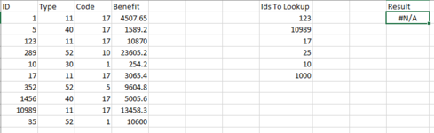
I am running into an issue with an excel formula. So the point is to sum Column D (in cell K2) only for the numbers that exist in column H, and only for those numbers that have Column B = 11 and Column C = 17.
I was able to partially get there with an array formula, but the problem is since the "arrays" are of different dimensions I am still getting an NA error.

I have also tried utilizing SUMIFS but that didn't work, at least the way I tried to use it. I also thought about SUMPRODUCT but I am not sure if that will work either due to the difference in "array" sizes.

Is there a way to make this work with one single formula? (I know this can be done by using a helper column and a simple SUMIFS but I was wondering if it can be done without adding clutter).

Attached an image with my sample data. Formula in K2 is the following: {=SUM(IF((ISNUMBER(MATCH(H2:H7,A2:A11,0)))*(B2:B11=11)*(C2:C11=17),D2:D11))}

 

[Fluff]

How about

=SUM(SUMIFS(D:D,A:A,H2:H7))

 

[jasonb75]

From your image I would think that you simply want

=SUMPRODUCT(SUMIFS(D2:D11,A2:A11,H2:H7,B2:B11,11,C2:C11,17))

edit:- for your information, your array formula would work if you swapped the 2 ranges in match, {=SUM(IF((ISNUMBER(MATCH(A2:A11,H2:H7,0)))*(B2:B11=11)*(C2:C11=17),D2:D11))} so that the array which is not the same size as the rest is the match range instead of the criteria.

 

[Martunis99]

@Fluff that has to be entered as an array function though, right? If I try to enter it as a normal function it just returns the value of the first ID. Either way, as an array function it works so thank you!

@jasonb75 that one absolutely works, thank you! And I changed my formula and it does indeed work. Makes sense, if the lookup value is the bigger array, no chance of getting NAs anymore. Good idea! I like your and @Fluff 's idea much better though. Much simpler.

Thank you guys so much!

 

[Fluff]

@Fluff that has to be entered as an array function though, right?

Very possibly, as CSE entry is not required with 365 or 2021, I can't always remember what needs CSE & what doesn't.

 

[Martunis99]

Very possibly, as CSE entry is not required with 365 or 2021, I can't always remember what needs CSE & what doesn't.

Right! I forget 365 has a few cool new tricks.

Thank you for your input!

 

[Fluff]

Glad we could help & thanks for the feedback.