Sum unique values

[creative999]

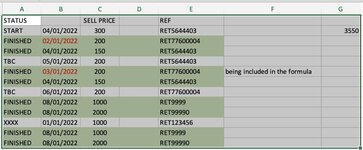
Trying to do a sum of column B if col A = Finished (and where col c value is unique).
For example

'Finished' should = 350

Book3
	A	B	C
1	STATUS	SELL PRICE	REF
2	START	300	RET5644403
3	FINISHED	200	RET77600004
4	FINISHED	150	RET5644403
5	TBC	200	RET5644403
6	FINISHED	200	RET77600004
7	FINISHED	150	RET5644403
8	TBC	200	RET77600004
Sheet2

 

[Fluff]

Unique is just that, a one of a kind, the distinct values are those you will get if you use the unique function on col C.

 

[igold]

ok

 

[igold]

Ok, there are no unique values and two distinct values. How does that make the Post any clearer when referencing that against Column A as requested by the OP.

 

[creative999]

When there are duplicates in column C, will the corresponding values in B also be the same? So, B3 will be the same as B6 because the C columns are the same?

yes, which is why I only want to sum where col c has distinct value else I’ll be double counting

 

[kweaver]

What about this?

Book5
	A	B	C	D	E
1	STATUS	SELL PRICE	REF
2	START	300	RET5644403		3350
3	FINISHED	200	RET77600004
4	FINISHED	150	RET5644403
5	TBC	200	RET5644403
6	FINISHED	200	RET77600004
7	FINISHED	150	RET5644403
8	TBC	200	RET77600004
9	FINISHED	1000	RET9999
10	FINISHED	2000	RET99990
11	XXXX	1000	RET123456
12	FINISHED	1000	RET9999
13	FINISHED	2000	RET99990
Sheet1

Cell Formulas
Range	Formula
E2	E2	=SUM(INDEX(UNIQUE(FILTER(A2:C13,A2:A13="FINISHED")),,2))

 

[creative999]

Worked perfectly. Thank you so much !!!

 

[creative999]

Found a problem with the formula. The actual data has additional columns between A-B and B-C (date / timestamp) which i didnt think were necessary to include here. In most cases the timestamp is the same for the REF and 'Finished' but there are some exceptions where its different and the calculation is picking this as unique and adding the SELL PRICE value to the final sum calculation. How can i ignore the timestamp?

 

[creative999]

Example here:

unique example.xlsx
	A	B	C	D	E	F	G
1	STATUS		SELL PRICE		REF
2	START	1/4/22	300		RET5644403		3550
3	FINISHED	1/2/22	200		RET77600004
4	FINISHED	1/4/22	150		RET5644403
5	TBC	1/5/22	200		RET5644403
6	FINISHED	1/3/22	200		RET77600004	this is being included in the formula
7	FINISHED	1/4/22	150		RET5644403
8	TBC	1/6/22	200		RET77600004
9	FINISHED	1/8/22	1000		RET9999
10	FINISHED	1/8/22	2000		RET99990
11	XXXX	1/1/22	1000		RET123456
12	FINISHED	1/8/22	1000		RET9999
13	FINISHED	1/8/22	2000		RET99990
Sheet3

Cell Formulas
Range	Formula
G2	G2	=SUM(INDEX(UNIQUE(FILTER(A2:E13,A2:A13="FINISHED")),,3))

 

[Fluff]

Do you have any data in col D?

 

[creative999]

Do you have any data in col D?

Yes there will be and also other columns. In the actual sheet, the ref id goes in col Y