Hi All
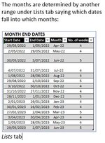
I just can't get my SUMIF to work here. Perhaps someone can see the error? I would like to sum the totals of actual spends across months but those 'months' don't fall completely inside the calendar month (it's the financial year whereby months have 4 or 5 weeks in them), so I need to do a lookup of some sort as week to determine what date falls within what month.
It works if I only use one criterion, that is the values are taken from the "Forecast Costs" cells but that adds up all of the values. As soon as I try to put in the month criteria, I get $0.00.
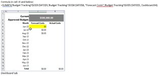
Please see attached. I want to sum totals if they fall under "Forecasted Costs" and by Month in the Budget Tracking tab onto the Dashboard tab - the month is to match 'Dashboard'!J4 and below.
Dashboard tab:
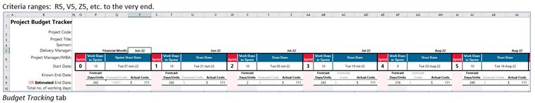
Budget tracking tab:
Lists tab:
I just can't get my SUMIF to work here. Perhaps someone can see the error? I would like to sum the totals of actual spends across months but those 'months' don't fall completely inside the calendar month (it's the financial year whereby months have 4 or 5 weeks in them), so I need to do a lookup of some sort as week to determine what date falls within what month.
It works if I only use one criterion, that is the values are taken from the "Forecast Costs" cells but that adds up all of the values. As soon as I try to put in the month criteria, I get $0.00.
Please see attached. I want to sum totals if they fall under "Forecasted Costs" and by Month in the Budget Tracking tab onto the Dashboard tab - the month is to match 'Dashboard'!J4 and below.
Dashboard tab:
| Budget Tracker example.xlsx | |||||
|---|---|---|---|---|---|
| I | J | K | |||
| 2 | Current Approved Budget: | $500,000.00 | |||
| 3 | Month | Forecast Costs | Actual Costs | ||
| 4 | Jun-22 | $0.00 | |||
| 5 | Jul-22 | $0.00 | |||
| 6 | Aug-22 | $0.00 | |||
| 7 | Sep-22 | ||||
| 8 | Oct-22 | ||||
| 9 | Nov-22 | ||||
| 10 | Dec-22 | ||||
| 11 | Jan-23 | ||||
| 12 | Feb-23 | ||||
| 13 | Mar-23 | ||||
| 14 | Apr-23 | ||||
| 15 | May-23 | ||||
| 16 | Jun-23 | ||||
| 17 | Total | $0.00 | $0.00 | ||
Dashboard | |||||
| Cell Formulas | ||
|---|---|---|
| Range | Formula | |
| J4:J6 | J4 | =SUMIFS('Budget Tracking'!$O$9:$XFD$9,'Budget Tracking'!$O$8:$XFD$8, "Forecast Costs",'Budget Tracking'!$O$5:$XFD$5, Dashboard!I4) |
| J17:K17 | J17 | =SUM(J5:J16) |
Budget tracking tab:
| Budget Tracker example.xlsx | ||||||||||||||||||||||||||
|---|---|---|---|---|---|---|---|---|---|---|---|---|---|---|---|---|---|---|---|---|---|---|---|---|---|---|
| O | P | Q | R | S | T | U | V | W | X | Y | Z | AA | AB | AC | AD | AE | AF | AG | AH | AI | AJ | AK | AL | |||
| 5 | Financial Month: | Jun-22 | Jun-22 | Jul-22 | Jul-22 | Aug-22 | Aug-22 | |||||||||||||||||||
| 6 | Sprint | Work Days in Sprint | Sprint Start Date | Sprint | Work Days in Sprint | Start Date | Sprint | Work Days in Sprint | Start Date | Sprint | Work Days in Sprint | Start Date | Sprint | Work Days in Sprint | Start Date | Sprint | Work Days in Sprint | Start Date | ||||||||
| 7 | 0 | 10 | Tue 07-Jun-22 | 1 | 10 | Tue 21-Jun-22 | 2 | 10 | Tue 05-Jul-22 | 3 | 10 | Tue 19-Jul-22 | 4 | 9 | Tue 02-Aug-22 | 5 | 10 | Tue 16-Aug-22 | ||||||||
| 8 | Forecast Days/Units | Forecast Costs | Actual Costs | Forecast Days/Units | Forecast Costs | Actual Costs | Forecast Days/Units | Forecast Costs | Actual Costs | Forecast Days/Units | Forecast Costs | Actual Costs | Forecast Days/Units | Forecast Costs | Actual Costs | Forecast Days/Units | Forecast Costs | Actual Costs | ||||||||
| 9 | 242 | #REF! | $ 111 | 242 | $ - | $ 111 | 2 | $ - | $ 111 | 242 | $ - | $ 111 | 216 | $ - | $ 111 | 240 | $ - | $ 111 | ||||||||
Budget Tracking | ||||||||||||||||||||||||||
| Cell Formulas | ||
|---|---|---|
| Range | Formula | |
| R5,AL5,AH5,AD5,Z5,V5 | R5 | =LOOKUP(Q7,MonthEndDates[Start Date],MonthEndDates[Month]) |
| P7,AJ7,AF7,AB7,X7,T7 | P7 | =IF(Q$7="","",NETWORKDAYS(Q$7,(Q$7+13),Holidays[Date])) |
| Q7 | Q7 | =IF($C$7="","",$C$7) |
| S7,AI7,AE7,AA7,W7 | S7 | =O7+1 |
| U7,AK7,AG7,AC7,Y7 | U7 | =Q7+14 |
| AJ9:AK9,AF9:AG9,AB9:AC9,X9:Y9,T9:U9,P9:Q9 | P9 | =SUM(P13:P1010) |
| R9,AL9,AH9,AD9,Z9,V9 | R9 | =SUM(R11:R1010) |
Lists tab:
| Budget Tracker example.xlsx | ||||||
|---|---|---|---|---|---|---|
| G | H | I | J | |||
| 1 | MONTH END DATES | |||||
| 2 | Start Date | End Date | Month | No. of weeks | ||
| 3 | 29/03/2022 | 1/05/2022 | Apr-22 | 4 | ||
| 4 | 2/05/2022 | 29/05/2022 | May-22 | 4 | ||
| 5 | 30/05/2022 | 3/07/2022 | Jun-22 | 5 | ||
| 6 | 4/07/2022 | 31/07/2022 | Jul-22 | 4 | ||
| 7 | 1/08/2022 | 28/08/2022 | Aug-22 | 4 | ||
| 8 | 29/08/2022 | 2/10/2022 | Sep-22 | 5 | ||
| 9 | 3/10/2022 | 30/10/2022 | Oct-22 | 4 | ||
| 10 | 31/10/2022 | 27/11/2022 | Nov-22 | 4 | ||
| 11 | 28/11/2022 | 1/01/2023 | Dec-22 | 5 | ||
| 12 | 2/01/2023 | 29/01/2023 | Jan-23 | 4 | ||
| 13 | 30/01/2023 | 26/02/2023 | Feb-23 | 4 | ||
| 14 | 27/02/2023 | 2/04/2023 | Mar-23 | 5 | ||
| 15 | 3/04/2023 | 30/04/2023 | Apr-23 | 4 | ||
| 16 | 1/05/2023 | 28/05/2023 | May-23 | 4 | ||
| 17 | 29/05/2023 | 2/07/2023 | Jun-23 | 5 | ||
Lists | ||||||
| Cell Formulas | ||
|---|---|---|
| Range | Formula | |
| G4:G17 | G4 | =H3+1 |