now i have the file - much easier to work - with - having an initial look - following comments
(i'm going to be away for a few days now after tonight, and wont be online till probably Sunday 6th Nov)
A countif or 2 should do this
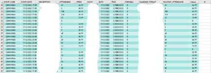
the time in B13 also has a date - so that needs to be removed
I have used in A13
B13-INT(B13) - this now just gets the time and can be used in a count
so we have
=COUNTIFS(ATTENDANCE!E:E,'2018 1 Hour Counts'!A7,ATTENDANCE!F:F,'2018 1 Hour Counts'!A13, ATTENDANCE!J:J,F13)
Where F13 is 74.99 ,
which in F14 = 1 and matches a FILTER on the data
and also
=COUNTIFS(ATTENDANCE!E:E,'2018 1 Hour Counts'!A7,ATTENDANCE!F:F,'2018 1 Hour Counts'!A13, ATTENDANCE!J:J,G13)
G13 = 39.99
which in G14 = 0 and matches a FILTER on the data
As i test , I tried 34.99 where you have 1 entry and it worked
treid some of the other VIP and got zero - so I would need to add some dummy data and check those
I have split out across a few columns - just to see the working
you can add those together
=COUNTIFS(ATTENDANCE!E:E,'2018 1 Hour Counts'!A7,ATTENDANCE!F:F,'2018 1 Hour Counts'!A13, ATTENDANCE!J:J,74.99)+
=COUNTIFS(ATTENDANCE!E:E,'2018 1 Hour Counts'!A7,ATTENDANCE!F:F,'2018 1 Hour Counts'!A13, ATTENDANCE!J:J,39.99)
Or we can play with a array - and use 1 function with or sumproduct
BUT lets just start here and make sure this works OK for you
and then revise as we go along
so i think
=COUNTIFS(ATTENDANCE!$E:$E,'2018 1 Hour Counts'!A7,ATTENDANCE!$F:$F,'2018 1 Hour Counts'!A13, ATTENDANCE!$J:$J,74.99)+
=COUNTIFS(ATTENDANCE!$E:4E,'2018 1 Hour Counts'!A7,ATTENDANCE!$F:$F,'2018 1 Hour Counts'!A13, ATTENDANCE!$J:$J,39.99)
will work and you just need to change
A7 and A13 for the different reference for the Dates and times
I need to see why in the time you need the date and if i can sort that

www.dropbox.com
i'll look into why just using K1 - is not working , in the cell
do you need to add the date and then just display the time ????
I guess we could just use that cell and use a different column which has the date and the time in