SumIFs based on multiple conditions and multiply by a value if certain text present

[questforexcel]

Hi All,

I am hoping you could help on this one.

I need my formula to search 2 columns in excel.

One column is based on the asset type. The other is based on the currency.

I need my formula to return the total by asset type and in SGD equivalent currency.

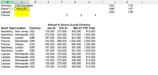
From my larger data set, i am trying this formula = SUMIFS($B$35:$T$39,L$35:L$39,$C8,I$35:I$39,"USD",I$35:I$39,"CAD",I$35:I$39,"GBP") but it returns the value error.

The above formula is not complete. I want my formula to multiply by the USD FX rate, if asset is in USD, GBP FX rate, if in GBP and CAD FX Rate, if in CAD.

Could you please help guide me on how to use a formula which can sum if based on the multiple criterias and multiply the individual USD, CAD, GBP numbers while summing them up. So that I can arrive at the SGD Equivalent number.

Is this possible?

I am not able to download or enable XL2BB on laptop. Apologies for any inconvenience.

						USD	1.35​
						GBP	1.67​
						CAD	1.00​
Asset Type	Location	Name of Asset	Currency	Amount	SGD
Machinery	New Jersey	Generator	USD	135,000	100,000
Machinery	Minneapolis	UPS	USD	270,000	200,000
Laptop	London		GBP	167,000	100,000
Buildings	Manchester	Tower	GBP	334,000	100,000
Land	Ottawa		CAD	200,000	200,000
			Total in Reporting Currency	1,106,000
			Total in SGD Equivalent	700,000

 

[Sufiyan97]

Hi
Sorry, Not clear with your query
Can you post some data on how your data looks like including all the ranges you have used in the formula.

 

[questforexcel]

Hi,

Thank you for your response.

I have records of data assets across different locations in different source currencies.

I am looking to find a way to sum the total by asset type and the SGD equivalent currency.

In order for it to be shown in the SGD Equivalent currency, i think I would need the formula to lookup the foreign currency values and multiply by them by their respective FX rate to SGD.

This is the formula that I have included below. But I have not been able to multiply the individual USD, GBP, CAD amounts by their respective exchange rates in the formula. May be sumifs isnt the right formula here?

Would appreciate any help / guidance here. Thank you very much

=SUMIFS($B$9:$H$20,B$9:B$20,B$2,H$9:H$20,J$1,H$9:H$20,J$2,H$9:H$20,J$3)

Summary	SGD Equivalent						USD	1.35​
Machinery	#VALUE!​							GBP	1.67​
Laptops								CAD	1.00​
Fixtures				2​	3​	4​
			Amount in Source (Local) Currency
Asset Type	Location	Currency	Jan-23​	Feb-23​	Mar-23​	YTD Total
Machinery	New Jersey	USD	135,000	270,000	405,000	810,000
Machinery	Minneapolis	USD	270,000	540,000	810,000	1,620,000
Fixtures	London	GBP	167,000	334,000	501,000	1,002,000
Fixtures	Manchester	GBP	334,000	668,000	1,002,000	2,004,000
Fixtures	Ottawa	CAD	200,000	400,000	600,000	1,200,000
Machinery	London	GBP	167,000	334,000	501,000	1,002,000
Machinery	London	GBP	167,000	334,000	501,000	1,002,000
Laptops	Minneapolis	USD	135,000	270,000	405,000	810,000
Laptops	Minneapolis	USD	135,000	270,000	405,000	810,000
Laptops	Minneapolis	USD	135,000	270,000	405,000	810,000
Laptops	Minneapolis	USD	135,000	270,000	405,000	810,000
Laptops	Minneapolis	USD	135,000	270,000	405,000	810,000

 

[ExceLoki]

i'm assuming you are looking for each summary as ytd?
if you can add a single helper column as i have the YTD SGD Equivalent shown below, then this may work for you:

Book1
	A	B	C	D	E	F	G	H	I	J
1	Summary	SGD Equivalent							USD	1.35
2	Machinery	3000000.00							GBP	1.67
3	Laptops	3000000.00							CAD	1.00
4	Fixtures	3000000.00
5					Amount in Source (Local) Currency
6	Asset Type	Location	Currency	YTD SGD Equivalent	Jan-23	Feb-23	Mar-23	YTD Total
7	Machinery	New Jersey	USD	600000.00	135000.00	270000.00	405000.00	810000.00
8	Machinery	Minneapolis	USD	1200000.00	270000.00	540000.00	810000.00	1620000.00
9	Fixtures	London	GBP	600000.00	167000.00	334000.00	501000.00	1002000.00
10	Fixtures	Manchester	GBP	1200000.00	334000.00	668000.00	1002000.00	2004000.00
11	Fixtures	Ottawa	CAD	1200000.00	200000.00	400000.00	600000.00	1200000.00
12	Machinery	London	GBP	600000.00	167000.00	334000.00	501000.00	1002000.00
13	Machinery	London	GBP	600000.00	167000.00	334000.00	501000.00	1002000.00
14	Laptops	Minneapolis	USD	600000.00	135000.00	270000.00	405000.00	810000.00
15	Laptops	Minneapolis	USD	600000.00	135000.00	270000.00	405000.00	810000.00
16	Laptops	Minneapolis	USD	600000.00	135000.00	270000.00	405000.00	810000.00
17	Laptops	Minneapolis	USD	600000.00	135000.00	270000.00	405000.00	810000.00
18	Laptops	Minneapolis	USD	600000.00	135000.00	270000.00	405000.00	810000.00
Sheet2

Cell Formulas
Range	Formula
B2:B4	B2	=SUMIF($A$7:$A$18,A2,$D$7:$D$18)
D7:D18	D7	=H7/VALUE(LEFT(VLOOKUP(C7,$I$1:$J$3,2,FALSE),4))
H7:H18	H7	=SUM(E7:G7)

 

[questforexcel]

Thank you very much for your time and help.

I may not have the possibility for adding further columns. There would be a YTD column, a current year estimate column and next year outlook column. Which are currently hidden.

So I would need the formula to look this up on the summary section b2:B4 above.

Is there anyway that could be done? Thank you

 

[Sufiyan97]

Hi I tried to do it without helper column, but strangly it works on 365 but not in Excel 2013.

@Fluff Please do you have any idea why is that?

SUMPRODUCT - Copy (2).xlsx
	A	B	C	D	E	F	G	H	I	J	K
1	Summary	SGD Equivalent	With 365	With Excel 2013					USD	1.35
2	Machinery		3000000	3284444.444					GBP	1.67
3	Laptops		3000000	3000000					CAD	1
4	Fixtures		3000000	3115555.556
5					Amount in Source (Local) Currency
6	Asset Type	Location	Currency	YTD SGD Equivalent	23-Jan	23-Feb	23-Mar	YTD Total
7	Machinery	New Jersey	USD		135000	270000	405000	810000
8	Machinery	Minneapolis	USD		270000	540000	810000	1620000
9	Fixtures	London	GBP		167000	334000	501000	1002000
10	Fixtures	Manchester	GBP		334000	668000	1002000	2004000
11	Fixtures	Ottawa	CAD		200000	400000	600000	1200000
12	Machinery	London	GBP		167000	334000	501000	1002000
13	Machinery	London	GBP		167000	334000	501000	1002000
14	Laptops	Minneapolis	USD		135000	270000	405000	810000
15	Laptops	Minneapolis	USD		135000	270000	405000	810000
16	Laptops	Minneapolis	USD		135000	270000	405000	810000
17	Laptops	Minneapolis	USD		135000	270000	405000	810000
18	Laptops	Minneapolis	USD		135000	270000	405000	810000
19
20
Sheet10

Cell Formulas
Range	Formula
C2:C4	C2	=SUMPRODUCT($H$7:$H$18/VLOOKUP($C$7:$C$18,$I$1:$J$3,2,FALSE)*($A$7:$A$18=A2))
D2:D4	D2	=SUMPRODUCT($H$7:$H$18/VLOOKUP($C$7:$C$18,$I$1:$J$3,2,FALSE)*($A$7:$A$18=A2))
H7:H18	H7	=SUM(E7:G7)
Press CTRL+SHIFT+ENTER to enter array formulas.

Named Ranges
Name	Refers To	Cells
CAD	=Sheet10!$I$3:$J$3	C2:D4
GBP	=Sheet10!$I$2:$J$2	C2:D4
USD	=Sheet10!$I$1:$J$1	C2:D4

 

[ExceLoki]

multiple posts solutions.xlsx
	A	B	C	D	E	F	G	H	I	J
1	Summary	SGD Equivalent							USD	1.35
2	Machinery	3000000.00							GBP	1.67
3	Laptops	3000000.00							CAD	1.00
4	Fixtures	3000000.00
5					Amount in Source (Local) Currency
6	Asset Type	Location	Currency		Jan-23	Feb-23	Mar-23	YTD Total
7	Machinery	New Jersey	USD		135000.00	270000.00	405000.00	810000.00
8	Machinery	Minneapolis	USD		270000.00	540000.00	810000.00	1620000.00
9	Fixtures	London	GBP		167000.00	334000.00	501000.00	1002000.00
10	Fixtures	Manchester	GBP		334000.00	668000.00	1002000.00	2004000.00
11	Fixtures	Ottawa	CAD		200000.00	400000.00	600000.00	1200000.00
12	Machinery	London	GBP		167000.00	334000.00	501000.00	1002000.00
13	Machinery	London	GBP		167000.00	334000.00	501000.00	1002000.00
14	Laptops	Minneapolis	USD		135000.00	270000.00	405000.00	810000.00
15	Laptops	Minneapolis	USD		135000.00	270000.00	405000.00	810000.00
16	Laptops	Minneapolis	USD		135000.00	270000.00	405000.00	810000.00
17	Laptops	Minneapolis	USD		135000.00	270000.00	405000.00	810000.00
18	Laptops	Minneapolis	USD		135000.00	270000.00	405000.00	810000.00
sumifs conversion

Cell Formulas
Range	Formula
B2:B4	B2	=(SUMIFS($H$7:$H$18,$C$7:$C$18,$I$1,$A$7:$A$18,A2)/VALUE(LEFT(VLOOKUP($I$1,$I$1:$J$3,2,FALSE),4)))+(SUMIFS($H$7:$H$18,$C$7:$C$18,$I$2,$A$7:$A$18,A2)/VALUE(LEFT(VLOOKUP($I$2,$I$1:$J$3,2,FALSE),4)))+(SUMIFS($H$7:$H$18,$C$7:$C$18,$I$3,$A$7:$A$18,A2)/VALUE(LEFT(VLOOKUP($I$3,$I$1:$J$3,2,FALSE),4)))
H7:H18	H7	=SUM(E7:G7)

 

[Sufiyan97]

Hi @ExceLoki

Do you have a specific reason putting VALUE and LEFT, just wanted to know

I just removed it and it works same.

Products.xlsx
	A	B	C	D	E	F	G	H	I	J	K
1	Summary	SGD Equivalent							USD	1.35
2	Machinery	3000000							GBP	1.67
3	Laptops	3000000							CAD	1
4	Fixtures	3000000
5					Amount in Source (Local) Currency
6	Asset Type	Location	Currency		23-Jan	23-Feb	23-Mar	YTD Total
7	Machinery	New Jersey	USD		135000	270000	405000	810000
8	Machinery	Minneapolis	USD		270000	540000	810000	1620000
9	Fixtures	London	GBP		167000	334000	501000	1002000
10	Fixtures	Manchester	GBP		334000	668000	1002000	2004000
11	Fixtures	Ottawa	CAD		200000	400000	600000	1200000
12	Machinery	London	GBP		167000	334000	501000	1002000
13	Machinery	London	GBP		167000	334000	501000	1002000
14	Laptops	Minneapolis	USD		135000	270000	405000	810000
15	Laptops	Minneapolis	USD		135000	270000	405000	810000
16	Laptops	Minneapolis	USD		135000	270000	405000	810000
17	Laptops	Minneapolis	USD		135000	270000	405000	810000
18	Laptops	Minneapolis	USD		135000	270000	405000	810000
19
Sheet11

Cell Formulas
Range	Formula
B2:B4	B2	=(SUMIFS($H$7:$H$18,$C$7:$C$18,$I$1,$A$7:$A$18,A2)/VLOOKUP($I$1,$I$1:$J$3,2,FALSE)+(SUMIFS($H$7:$H$18,$C$7:$C$18,$I$2,$A$7:$A$18,A2)/VLOOKUP($I$2,$I$1:$J$3,2,FALSE))+(SUMIFS($H$7:$H$18,$C$7:$C$18,$I$3,$A$7:$A$18,A2)/VLOOKUP($I$3,$I$1:$J$3,2,FALSE)))
H7:H18	H7	=SUM(E7:G7)

 

[ExceLoki]

i had left in there as i was trying another way to solve, it's not needed in the final solution... good catch

multiple posts solutions.xlsx
	A	B	C	D	E	F	G	H	I	J
1	Summary	Me							USD	1.35
2	Machinery	3000000.00							GBP	1.67
3	Laptops	3000000.00							CAD	1.00
4	Fixtures	3000000.00
5					Amount in Source (Local) Currency
6	Asset Type	Location	Currency		Jan-23	Feb-23	Mar-23	YTD Total
7	Machinery	New Jersey	USD		135000.00	270000.00	405000.00	810000.00
8	Machinery	Minneapolis	USD		270000.00	540000.00	810000.00	1620000.00
9	Fixtures	London	GBP		167000.00	334000.00	501000.00	1002000.00
10	Fixtures	Manchester	GBP		334000.00	668000.00	1002000.00	2004000.00
11	Fixtures	Ottawa	CAD		200000.00	400000.00	600000.00	1200000.00
12	Machinery	London	GBP		167000.00	334000.00	501000.00	1002000.00
13	Machinery	London	GBP		167000.00	334000.00	501000.00	1002000.00
14	Laptops	Minneapolis	USD		135000.00	270000.00	405000.00	810000.00
15	Laptops	Minneapolis	USD		135000.00	270000.00	405000.00	810000.00
16	Laptops	Minneapolis	USD		135000.00	270000.00	405000.00	810000.00
17	Laptops	Minneapolis	USD		135000.00	270000.00	405000.00	810000.00
18	Laptops	Minneapolis	USD		135000.00	270000.00	405000.00	810000.00
sumifs conversion

Cell Formulas
Range	Formula
B2:B4	B2	=SUMIFS($H$7:$H$18,$C$7:$C$18,$I$1,$A$7:$A$18,A2)/(VLOOKUP($I$1,$I$1:$J$3,2,FALSE))+(SUMIFS($H$7:$H$18,$C$7:$C$18,$I$2,$A$7:$A$18,A2)/(VLOOKUP($I$2,$I$1:$J$3,2,FALSE)))+(SUMIFS($H$7:$H$18,$C$7:$C$18,$I$3,$A$7:$A$18,A2)/(VLOOKUP($I$3,$I$1:$J$3,2,FALSE)))
H7:H18	H7	=SUM(E7:G7)

 

[Sufiyan97]

@questforexcel you should mark @ExceLoki 's formula in post #9 as a solution.