SUMIFS doesnot work with VSTACK and CHOOSECOLS?

[ErikHorsthuis]

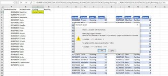
I am testing the new dynamic array functions (CHOOSECOLS and VSTACK) and I am trying to combine them with SUMIFS. I am trying to display in cell C2:D22 with SUMIFS the number of kudos from the respective student and sport. However, Excel does not allow up this formula. If I just run the SUMIFS formula on a table then of course it works. I'm afraid I'm overlooking something. Does anyone see what I am doing wrong? Thanks! I know that there are all kind of other approaches to solve this, I just want to know what is wrong in the formula.

=SUMIFS(CHOOSECOLS(VSTACK(Cycling,Running),4),CHOOSECOLS(VSTACK(Cycling,Running),1),A2#,CHOOSECOLS(VSTACK(Cycling,Running),3),C1#)

 

[bstrib]

I encountered this issue also but this was my solution matching your formula:

=map(a2#,c1#,lambda(a,b,sumproduct(--(choosecols(vstack(cycling,running),1)=a)*(choosecols(vstack(cycling,running),3)=b),choosecols(cycling,running),4)))))

Map function is needed here as you have a multi condition, a single condition would only need a byrow/bycol function.

Hope that works for you.

Hi fatalcry,

I may be late in this thread, but I really liked your very logical "MAP" function suggestion and tried it out. But I only get one correct result in the results array(1,1) cell, and #NA's for the rest of the array. I can separately use sumproduct and manually map it thru the results array - which gives me all correct answers - so I'm sure the core is working correctly. Have tried all kinds of things to get the Boolean array working correctly - but without success...

So this is really just a quick query to ask whether you actually got it working?

I attach here a copy of my dummy setup, and my separate manual mapping using the SUMPRODUCT function. Appreciate any wisdom you might have, or if you see I've done something silly that's easily fixed!!

[Note: I'm new to these types of forums, so apologies in advance if my approach here is incorrect or a bit clumsy, or I'm supposed to start a new thread...]

 

[Fluff]

How about

=SUMIFS(D2:D11,B2:B11,K3#,C2:C11,L2#)

 

[bstrib]

How about

=SUMIFS(D2:D11,B2:B11,K3#,C2:C11,L2#)

Dear "Fluff"

You're a STAR! I had played with the SUMIFS function earlier, but in hindsight, suspect I stupidly forgot to "transpose" the Divisions vector.

It now all works brilliantly, and I now have a complete "spillable" report in a single formula that summarises the data in two dimensions.

Don't understand why the MAP function doesn't get to the same result - logically seems perfect for such mapping - I was quite enthused about this as a great new tool. Oh well - c'est la vie!!

Next challenge/study (...which is where I thought MAP would be excellent) is to see if I can take this into working with n-dimensional arrays that are dynamic...

If it's of interest, my updated little 2-D study now looks like this:

 

[Fluff]

As this is a new question it needs a new thread. Thanks

 

[fatalcry]

Hi fatalcry,

I may be late in this thread, but I really liked your very logical "MAP" function suggestion and tried it out. But I only get one correct result in the results array(1,1) cell, and #NA's for the rest of the array. I can separately use sumproduct and manually map it thru the results array - which gives me all correct answers - so I'm sure the core is working correctly. Have tried all kinds of things to get the Boolean array working correctly - but without success...

So this is really just a quick query to ask whether you actually got it working?

I attach here a copy of my dummy setup, and my separate manual mapping using the SUMPRODUCT function. Appreciate any wisdom you might have, or if you see I've done something silly that's easily fixed!!

[Note: I'm new to these types of forums, so apologies in advance if my approach here is incorrect or a bit clumsy, or I'm supposed to start a new thread...]

View attachment 89089

Hi bstrib,

Sorry for the late reply, whilst the above formula did work when I first made it I confirm it doesn't anymore.

I believe the map function fundamentals have changed, when I created this I was under the belief it could function in a multi directional query. This however does not appear to be the case now, MAP's are a single directional lambda function. So it needs to be either Horizontal or Vertical and not both.

However, this being said you can achieve the same result by using index formulas (a previous commenter had mentioned this). Here's an example of a let formula that converts an array into a range within the LET function.

=LET(
comp,INDEX(DROP(CHOOSECOLS(A1#,1),1),,1),
vend,INDEX(DROP(CHOOSECOLS(A1#,2),1),,1),
IFS(comp="Example1",MAXIFS(Table1[Due Date],Table1[Vendor],vend),comp="Example2",MAXIFS(Table2[Due Date],Table2[Vendor],vend)))

This is a formula used inside a real world example. The intent of the formula is to retrieve a due date from a list which can have duplicate vendor (supplier) names but under different companies.

When using index you only need to state column/row number depending on the direction you require, this will then convert the array into a range type allowing it to be utilized in sum/count/maxifs etc

Hope this helps.

 

[bstrib]

Hi bstrib,

Sorry for the late reply, whilst the above formula did work when I first made it I confirm it doesn't anymore.

I believe the map function fundamentals have changed, when I created this I was under the belief it could function in a multi directional query. This however does not appear to be the case now, MAP's are a single directional lambda function. So it needs to be either Horizontal or Vertical and not both.

However, this being said you can achieve the same result by using index formulas (a previous commenter had mentioned this). Here's an example of a let formula that converts an array into a range within the LET function.

=LET(
comp,INDEX(DROP(CHOOSECOLS(A1#,1),1),,1),
vend,INDEX(DROP(CHOOSECOLS(A1#,2),1),,1),
IFS(comp="Example1",MAXIFS(Table1[Due Date],Table1[Vendor],vend),comp="Example2",MAXIFS(Table2[Due Date],Table2[Vendor],vend)))

This is a formula used inside a real world example. The intent of the formula is to retrieve a due date from a list which can have duplicate vendor (supplier) names but under different companies.

When using index you only need to state column/row number depending on the direction you require, this will then convert the array into a range type allowing it to be utilized in sum/count/maxifs etc

Hope this helps.

Hi fatalcry,

Thanks kindly for coming back. Yes - I came to the same conclusion that MAP won't work in 2 or more dimensions...

I did find fairly nice ways to make it work, both with SUMIFS (...CELL K2 Formula - but only works with CELL RANGES as inputs - a SUMIFS limitation) and with MMULT (...CELL S2 Formula - which also works with named ranges). Both approaches put a whole "spillable" 2D report with headers and footers into a single LET function...

If it's of interest, I paste a copy of my little study model here...