Sumifs using multiple criteria

[willwall]

Hello
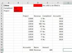
I am using sumifs to retrieve data from a table. On column "F" in the table i have a list of projects with transactions. On column "I" on the table I have the revenue generated from each project. What i want to do is use sumifs to calculate "all" revenues for all projects combined or in some cases calculate revenue for individual projects by typing in the project number in the criteria field.
Sum range = table
Criteria_range 1 = Column A
Criteria 22000 (project number) I would like some function here that can pick out "all" the projects and not just one.
If i could write e.g "All" or "22000" in the actual criteria cell it would be great. I tried a data validation drop down list which has no "All" function

 

[FormR]

Hi, you could try something like this, for example.

Book1
	A	B	C	D	E
1	Criteria Cell	Formula		Project	Revenue
2	All	650		22000	5
3				22000	15
4				22010	485
5				22020	45
6				22010	4
7				22000	77
8				22010	8
9				22020	7
10				22000	4
Sheet1

Cell Formulas
Range	Formula
B2	B2	=SUMIFS(E:E,D:D,IF(A2="All","<>",A2))

 

[jasonb75]

Another way would be

=IF(A2="All",SUM(E:E),SUMIF(D:D,A2,E:E))

Note that I've used SUMIF instead of SUMIFS as this method wouldn't work with more than 1 criteria range.

 

[willwall]

Hello Jasonb75
Both work great but I discovered that i need to take it one step further.
Above we wrote a formula for the revenue for "All" projects. I need to add in an account number to this so that "All" revenue for ledger number e.g 3000 gets summarised. Also there is a column in the table that shows completed projects "Yes or "No" which is also parts of the criteria. There are 2 cells marked in red where I usually type in the criteria. I attached a file to show what i mean. Maybe i have to use a pivottable for this, as there are a few filters involved. Really appreciate your help

 

[FormR]

Hi, not sure if I'm missing something but can't you just add the additional criteria into the SUMIFS() formula?

 

[jasonb75]

If you want the 'All' option for both red cells then you would need to use FormR's method, for example

=SUMIFS(D:D,C:C,IF(B3="All","<>",B3),E:E,IF(B2="All","<>",B2))

 

[willwall]

Yep this formula works and i added the extra sumif for the account number
=SUMIFS(D6:D14;C6:C14;IF(B3="All";"<>";B3);E6:E14;IF(B2="All";"<>";B2);F6:F14;C18)
Thanks guys for your help, this forum fanstastic.