Sumifs with multiple criteria placed in first tablerow, where criterias match

[Doge Robert]

Hello there.

I have a table with budgets for various suppliers and their locations (where they supply, what we're buying).
I also have three different ways of ordering their budgetary numbers into categories. (Suppliers version, our version and governments version)

I'm trying to do sums across the budgetary categories and then write the sum in the topmost row (in the sumcolumn for each category), which match all the criteria.

I've tried illustrating, what I need the sollution to look like in the table, with colorcoding to explain, how each sum is calculated.)

I've tried making a solution with array formulas and indirect (to get the dynamic cell ranges right), but I can't get it to work.

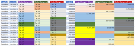
Example of sollution:
In the column BudgetCategory A Sum, I need to calculate the sum of the values in the budgetcolumn, corresponding to the the categories in the BudgetCategory A column for each matching set of supplier and location. So for Supplier A, Location A, Cat A B.
I can do it, but then the sum would appear in every row, where there is a matching set. So three times for Supplier A, Location A, Cat A B.

Is there a way to have the formula calculated for all matching sets but the result printed only in the topmost instance of each matching set?

I can't do it with pivottables, as I need the calculated sums for some other formulas first.

Note also that I'm using a table, as I'll have to add multiple suppliers and locations for each over time, so the ranges must be dynamic.

Is this even possible?

(I'm using Excel in Danish and working with confidential data, so I cannot upload an actual example)

I hope you can help me..

Kind Regards

Robert.

 

[Fluff]

Maybe something like

=IF(COUNTIFS(C$2:C2,C2)=1,SUMIFS(F:F,C:C,C2),"")

 

[Eric W]

In table nomenclature:

Book1 (version 1).xlsb
	C	D	E	F	G	H	I	J	K
1	Supplier	Locaton	Budget Category A	Budget Category B	Budget Category C	Budget	BudgetCategory A Sum	BudgetCategory B Sum	Budget Category C Sum
2	Supplier A	Location A	Cat A A	Cat B A	Cat C A	2000	2000	14235	3500
3	Supplier A	Location A	Cat A B	Cat B A	Cat C A	1500	12000
4	Supplier A	Location A	Cat A B	Cat B A	Cat C B	10000			20750
5	Supplier A	Location A	Cat A B	Cat B B	Cat C B	500		12450
6	Supplier A	Location A	Cat A C	Cat B B	Cat C B	7500	12980
7	Supplier A	Location A	Cat A C	Cat B B	Cat C B	2750
8	Supplier A	Location A	Cat A C	Cat B B	Cat C C	1800			1800
9	Supplier A	Location A	Cat A C	Cat B C	Cat C D	930		20430	21631
10	Supplier A	Location A	Cat A D	Cat B C	Cat C D	2000	19500
11	Supplier A	Location A	Cat A D	Cat B C	Cat C D	17500
12	Supplier A	Location A	Cat A E	Cat B D	Cat C D	201	6871	6136
13	Supplier A	Location A	Cat A E	Cat B D	Cat C D	1000
14	Supplier A	Location A	Cat A E	Cat B A	Cat C E	735			735
15	Supplier A	Location A	Cat A E	Cat B D	Cat C F	1715			1715
16	Supplier A	Location A	Cat A E	Cat B D	Cat C G	3220			3172.7
17	Supplier A	Location A	Cat A F	Cat B E	Cat C G	17.7	-47.3	52.7
18	Supplier A	Location A	Cat A F	Cat B E	Cat C G	35
19	Supplier A	Location A	Cat A F	Cat B B	Cat C G	-100
Sheet33

Cell Formulas
Range	Formula
I2:I19	I2	=IF(COUNTIF(INDEX([Budget Category A],1):[@[Budget Category A]],[@[Budget Category A]])=1,SUMIF([Budget Category A],[@[Budget Category A]],[Budget]),"")
J2:J19	J2	=IF(COUNTIF(INDEX([Budget Category B],1):[@[Budget Category B]],[@[Budget Category B]])=1,SUMIF([Budget Category B],[@[Budget Category B]],[Budget]),"")
K2:K19	K2	=IF(COUNTIF(INDEX([Budget Category C],1):[@[Budget Category C]],[@[Budget Category C]])=1,SUMIF([Budget Category C],[@[Budget Category C]],[Budget]),"")

Note that all 3 formulas can be combined into one, with INDIRECT and some manipulation, but I'm not so sure that's a good thing.

 

[Doge Robert]

Thank you both of you.

I need help tweaking the formulas a bit further though, as this has to happen once for each location for each supplier.

So once for Supplier A, Location A. Once for Supplier A, Location B. Once for Supplier B, Location A and so forth.

So two extra criterias.. I'm sorry that I explained that part poorly. You've both already been tremendously helpfull.

Fluff: So far, your formula sums all budgetary values across all locations and suppliers, but within the specific category and prints it at the first instance of said category.
How do I make it limit itself to the specific location of the specific supplier and then repeat the sum (and print) across each location of each supplier?

Eric W: Your formula sums the budgetary values within each specific category, across the first location, and prints it at the first instance of said category.
How do I make the formula repeat itself once for each location of each supplier?

Thank you both again. You've brought me a huge leap forward already.

 

[Fluff]

How about

Book1
	A	B	C	D	E	F	G	H	I
1	Supplier	Locaton	Budget Category A	Budget Category B	Budget Category C	Budget	BudgetCategory A Sum	BudgetCategory B Sum	Budget Category C Sum
2	Supplier A	Location A	Cat A A	Cat B A	Cat C A	2000	2000	13500	3500
3	Supplier A	Location A	Cat A B	Cat B A	Cat C A	1500	12000
4	Supplier A	Location A	Cat A B	Cat B A	Cat C B	10000			20750
5	Supplier A	Location A	Cat A B	Cat B B	Cat C B	500		10750
6	Supplier A	Location A	Cat A C	Cat B B	Cat C B	7500	10250
7	Supplier A	Location A	Cat A C	Cat B B	Cat C B	2750
8	Supplier B	Location A	Cat A C	Cat B B	Cat C C	1800	2730	1800	1800
9	Supplier B	Location A	Cat A C	Cat B C	Cat C D	930		18430	18631
10	Supplier B	Location B	Cat A D	Cat B C	Cat C D	2000	2000	2000	2000
11	Supplier B	Location A	Cat A D	Cat B C	Cat C D	17500	17500
12	Supplier B	Location A	Cat A E	Cat B D	Cat C D	201	201	201
13	Supplier C	Location A	Cat A E	Cat B D	Cat C D	1000	3450	2715	1000
14	Supplier C	Location A	Cat A E	Cat B A	Cat C E	735		735	735
15	Supplier C	Location A	Cat A E	Cat B D	Cat C F	1715			1715
16	Supplier C	Location B	Cat A E	Cat B D	Cat C G	3220	3220	3220	3172.7
17	Supplier C	Location B	Cat A F	Cat B E	Cat C G	17.7	-47.3	52.7
18	Supplier C	Location B	Cat A F	Cat B E	Cat C G	35
19	Supplier C	Location B	Cat A F	Cat B B	Cat C G	-100		-100
Sheet3

Cell Formulas
Range	Formula
G2:I19	G2	=IF(COUNTIFS($A$2:$A2,$A2,$B$2:$B2,$B2,C$2:C2,C2)=1,SUMIFS($F:$F,$A:$A,$A2,$B:$B,$B2,C:C,C2),"")

 

[Doge Robert]

How about

Book1
	A	B	C	D	E	F	G	H	I
1	Supplier	Locaton	Budget Category A	Budget Category B	Budget Category C	Budget	BudgetCategory A Sum	BudgetCategory B Sum	Budget Category C Sum
2	Supplier A	Location A	Cat A A	Cat B A	Cat C A	2000	2000	13500	3500
3	Supplier A	Location A	Cat A B	Cat B A	Cat C A	1500	12000
4	Supplier A	Location A	Cat A B	Cat B A	Cat C B	10000			20750
5	Supplier A	Location A	Cat A B	Cat B B	Cat C B	500		10750
6	Supplier A	Location A	Cat A C	Cat B B	Cat C B	7500	10250
7	Supplier A	Location A	Cat A C	Cat B B	Cat C B	2750
8	Supplier B	Location A	Cat A C	Cat B B	Cat C C	1800	2730	1800	1800
9	Supplier B	Location A	Cat A C	Cat B C	Cat C D	930		18430	18631
10	Supplier B	Location B	Cat A D	Cat B C	Cat C D	2000	2000	2000	2000
11	Supplier B	Location A	Cat A D	Cat B C	Cat C D	17500	17500
12	Supplier B	Location A	Cat A E	Cat B D	Cat C D	201	201	201
13	Supplier C	Location A	Cat A E	Cat B D	Cat C D	1000	3450	2715	1000
14	Supplier C	Location A	Cat A E	Cat B A	Cat C E	735		735	735
15	Supplier C	Location A	Cat A E	Cat B D	Cat C F	1715			1715
16	Supplier C	Location B	Cat A E	Cat B D	Cat C G	3220	3220	3220	3172.7
17	Supplier C	Location B	Cat A F	Cat B E	Cat C G	17.7	-47.3	52.7
18	Supplier C	Location B	Cat A F	Cat B E	Cat C G	35
19	Supplier C	Location B	Cat A F	Cat B B	Cat C G	-100		-100
Sheet3

Cell Formulas
Range	Formula
G2:I19	G2	=IF(COUNTIFS($A$2:$A2,$A2,$B$2:$B2,$B2,C$2:C2,C2)=1,SUMIFS($F:$F,$A:$A,$A2,$B:$B,$B2,C:C,C2),"")

This works flawlessly. Thank you very much.

Regards,

Robert.

 

[Fluff]

Glad we could help & thanks for the feedback.

 

[Eric W]

Here's the table nomenclature version:

Book1 (version 1).xlsb
	C	D	E	F	G	H	I	J	K
1	Supplier	Location	Budget Category A	Budget Category B	Budget Category C	Budget	Budget Category A Sum	Budget Category B Sum	Budget Category C Sum
2	Supplier A	Location A	Cat A A	Cat B A	Cat C A	2000	2000	13500	3500
3	Supplier A	Location A	Cat A B	Cat B A	Cat C A	1500	12000
4	Supplier A	Location A	Cat A B	Cat B A	Cat C B	10000			20750
5	Supplier A	Location A	Cat A B	Cat B B	Cat C B	500		10750
6	Supplier A	Location A	Cat A C	Cat B B	Cat C B	7500	10250
7	Supplier A	Location A	Cat A C	Cat B B	Cat C B	2750
8	Supplier B	Location A	Cat A C	Cat B B	Cat C C	1800	2730	1800	1800
9	Supplier B	Location A	Cat A C	Cat B C	Cat C D	930		18430	18631
10	Supplier B	Location B	Cat A D	Cat B C	Cat C D	2000	2000	2000	2000
11	Supplier B	Location A	Cat A D	Cat B C	Cat C D	17500	17500
12	Supplier B	Location A	Cat A E	Cat B D	Cat C D	201	201	201
13	Supplier C	Location A	Cat A E	Cat B D	Cat C D	1000	3450	2715	1000
14	Supplier C	Location A	Cat A E	Cat B A	Cat C E	735		735	735
15	Supplier C	Location A	Cat A E	Cat B D	Cat C F	1715			1715
16	Supplier C	Location B	Cat A E	Cat B D	Cat C G	3220	3220	3220	3172.7
17	Supplier C	Location B	Cat A F	Cat B E	Cat C G	17.7	-47.3	52.7
18	Supplier C	Location B	Cat A F	Cat B E	Cat C G	35
19	Supplier C	Location B	Cat A F	Cat B B	Cat C G	-100		-100
Sheet39

Cell Formulas
Range	Formula
I2:I19	I2	=IF(COUNTIFS(INDEX([Supplier],1):[@Supplier],[@Supplier],INDEX([Location],1):[@Location],[@Location],INDEX([Budget Category A],1):[@[Budget Category A]],[@[Budget Category A]])=1,SUMIFS([Budget],[Supplier],[@Supplier],[Location],[@Location],[Budget Category A],[@[Budget Category A]]),"")
J2:K19	J2	=IF(COUNTIFS(INDEX([Supplier],1):[@Supplier],[@Supplier],INDEX([Location],1):[@Location],[@Location],INDEX(Table2[#Data],1,COLUMN()-COLUMN([Supplier])-3):INDEX(Table2[#Data],ROW()-ROW(INDEX(Table2[#Data],1,1))+1,COLUMN()-COLUMN([Supplier])-3),INDEX(Table2[#Data],ROW()-ROW(INDEX(Table2[#Data],1,1))+1,COLUMN()-COLUMN([Supplier])-3))=1,SUMIFS([Budget],[Supplier],[@Supplier],[Location],[@Location],INDEX(Table2[#Data],0,COLUMN()-COLUMN([Supplier])-3),INDEX(Table2[#Data],ROW()-ROW(INDEX(Table2[#Data],1,1))+1,COLUMN()-COLUMN([Supplier])-3)),"")

I2 has the basic formula, using the appropriate column headers. J2 has a formula that you can copy into I2 and K2 that works in all columns, based on the first column being Supplier, and the Sum columns are 4 columns away from the corresponding category column. As you can see, it's pretty long and complicated, mainly because the table nomenclature doesn't have an easy way to say "this column". I'd stick with the I2 formula, and just change the headings as needed when you copy it to J2:K2.

Of course, Fluff's formula is shorter still, but this does have the benefit of automatically adjusting as you add rows to the table.