Summing a diagonally shaped area in a two-dimensional table

[longjohnsilver]

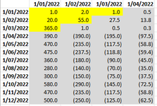
I am trying to sum across a two-dimensional array, where the cells I want to sum are in a "jagged" diagonal shape (refer to the yellow cells in the attached image).

I need the formula to be extendable, so that when I move across to the next date, the next "diagonal row" is then summed.

I have tried to use SUMPRODUCT formula (=SUMPRODUCT(B2:E13*(A2:A13<=A4)*(B1:E1<=D1)), but this is summing a square section of the table, not a "diagonally shaped" area. I have so far been unable to edit this formula to get the desired result.

Any ideas?

 

[jasonb75]

I'm assuming that the image shows the source data but I'm not following how you want the results laid out.

Taking a diagonal slice is possible but from what I can remember, it takes some fairly complex formulas to achieve. It would be useful if we could compare the source to the expected output for the first 3 rows / columns of data to be sure that we are on the same page.

 

[longjohnsilver]

I have manually calculated my expected outputs in row 2 as shown in the below image. I've color coded each of the outputs along with the new cells that are included in each output, note that the formula is cumulative, i.e. the 957.6 includes the red color plus all the other previous colors. Hope this helps.

 

[jasonb75]

I managed to make it a bit simpler than I expected, this looks correct as per your example but it does assume that the dates in the 3 ranges are all the same. Trying to match the dates in row 1 to those in row 4 and column A will be much more challenging. I have done something similar once before, but it was about 5 years ago on a different forum and I've not been able to find it for reference.

Try this formula in B2, then drag it right as needed.

=SUM(INDEX($B$5:$F$16,COLUMN(B2)-COLUMN($B2:B2)+1,COLUMN($B2:B2)-COLUMN($B2)+1),A2)

 

[longjohnsilver]

Perfect, that works well, thank you!