SUMPRODUCT WITH COLUMN SELECTION

[Phill032]

Hi all.. So i am using a sumproduct formula to sum and count data from a table.
However i have my criteria to meet in column A and along the top as headers i have month/Year.
I would like to have a drop down box to select a month/year on my report sheet so that the sumproduct would select that month/year column to read the data.
I can do the dropdown box so im only after the formula, any help or ideas would be greatly appreciated
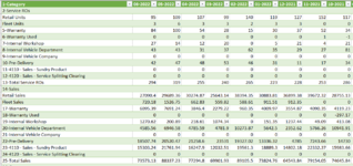
So ideally i would select 06-2022 for the month on my consolidated report and it would pull through all the data from the below for June, and if i select May the i get May's data.

Category	06-2022	05-2022	04-2022	03-2022	01-2022
Retail Units	95	103	100	82	56
Fleet Units	5	5	6	4	5

 

[KRice]

I'll assume your month-year headings are in B1:F1 on Sheet1 for a small example. And suppose your dropdown box selection is on Sheet2 in cells C2 where you might choose 06-2022.

=INDEX(Sheet1!$B$2:$F$30,,MATCH(Sheet2!$C$2,Sheet1!$B$1:$F$1,0))

would return rows 2:30 on Sheet1 from the column where the match is found with C2 on Sheet2.
...or are you asking for it to pull only the data for Fleet Units and Retails Units?

Edit: changed range in Index

Example with different sheet names:

MrExcel_20220617.xlsx
	A	B	C	D	E	F
1	Category \ Date	Jun-22	May-22	Apr-22	Mar-22	Feb-22
2	Service	1	5	4	7	9
3	Retail Units	8	6	3	5	5
4	Fleet Units	7	9	1	5	7
5	Other	4	1	3	2	1
Sheet6

MrExcel_20220617.xlsx
	C
1
2
3	May-22
4
5	6
6	9
7
8
Sheet7

Cell Formulas
Range	Formula
C5:C6	C5	=INDEX(Sheet6!$B$2:$F$5,{2;3},MATCH(C3,Sheet6!$B$1:$F$1,0))
Dynamic array formulas.

If you know the location of the Retail and Fleet rows, you could hardwire their row index positions into the formula as an array like this.

 

[Phill032]

I'll assume your month-year headings are in B1:F1 on Sheet1 for a small example. And suppose your dropdown box selection is on Sheet2 in cells C2 where you might choose 06-2022.

=INDEX(Sheet1!$A$2:$F$30,,MATCH(Sheet2!$C$2,Sheet1!$B$1:$F$1,0))

would return rows 2:30 on Sheet1 from the column where the match is found with C2 on Sheet2.
...or are you asking for it to pull only the data for Fleet Units and Retails Units?

As the data is pulled in through power query i have done a transpose of the table and i think this may have solved my problem.
I will have a go at your example above to see how it works

 

[KRice]

If you are bringing it in from PQ, and you don't need any other data from your main source, you could add some lines to the M-code that would delete everything but the month, Fleet, and Retail values. If you are bringing over more data and you know where the Retail and Fleet rows are, then the hardwired row index approach in the INDEX/MATCH formula in my last post is convenient. If you don't know the location of the Retail and Fleet rows, then more is needed to do this with a formula (e.g., another MATCH function to find the rows). What version of Excel are you using?

 

[Phill032]

If you are bringing it in from PQ, and you don't need any other data from your main source, you could add some lines to the M-code that would delete everything but the month, Fleet, and Retail values. If you are bringing over more data and you know where the Retail and Fleet rows are, then the hardwired row index approach in the INDEX/MATCH formula in my last post is convenient. If you don't know the location of the Retail and Fleet rows, then more is needed to do this with a formula (e.g., another MATCH function to find the rows). What version of Excel are you using?

Using 365, there are over 200 lines in each of the 2 reports that i need to consolidate.
Some of the criteria in the Category column are named the same, by doing a transpose it has eliminated this problem and i can utilise the month year as dropdown in column A.
The categories become the headers which are fixed into my main report anyway. Thanks for your help but i think i will just go with PQ doing the hard work for now.

 

[KRice]

Sounds good. Post back if you encounter any difficulties.