SUMs and VLookup Issues

[alphairri]

Link to Excel file: Diet (1).xlsx

I have a diet planner that I am trying to work with.
FOOD CATALOG sheet has all the macro information.
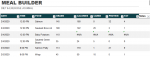
MEAL BUILDER sheet has the DATE, TIME, FOOD (from drop-down), and GRAMS eaten.
-Issue one: VLOOKUP is failing for random things. In the link, "Baby Potatoes" isn't being found in the FOOD CATALOG sheet, but it works if I just call it "Potatoes".
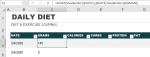
DAILY DIET sheet should add all info from the MEAL BUILDER sheet that has a matching date.
-Issue two: I've tried SUM with VLOOKUP and SUMIFS, but I haven't been able to get it to show more than one cell of data.

Any help is greatly appreciated!

 

[outlawdevil]

For Vlookup, can you check if they are same format? if they are, make sure you use absolute range for lookup array or use the whole column like =vlookup(D6,B:G,3,0) to get calorie

I would just go over the Sumif formula again to make sure you sum those correct. =sumif(range,criteria, sum_range) make sure to use absolute reference as well.

 

[Fluff]

Hi & welcome to MrExcel.
Can you please post the Vlookup formula that isn't working, along with what you have tried for issue 2

 

[alphairri]

Formula is F6 is
=VLOOKUP($D6,FoodCatalog,3)*$E6/100

Here is the FoodCatalog table

--
The strange thing is that if I change "Baby Potatoes" to "Potatoes", it works. The FOOD column (D) on MEAL BUILDER uses Data Validation from the FOOD column (B) on FOOD CATALOG.

 

[Fluff]

The Vlookup should be
=VLOOKUP($D6,FoodCatalog,3,0)*$E6/100
Otherwise you are doing an approximate match, in which case the lookup table must be sorted A-Z

 

[alphairri]

Thank you, Fluff! That fixed the Meal Builder portion.

The SUMIF that I last tried was
=SUMIF(MealBuilder,[@DATE],MealBuilder[@GRAMS])
First row is correct, but the second row doesn't.

The number should be 470 for 2/4/2020

 

[Fluff]

Ok, that formula should be
=SUMIF(MealBuilder[DATE],[@DATE],MealBuilder[GRAMS])

 

[alphairri]

Perfect!!!
Thank you so much for all your help!

 

[Fluff]

You're welcome & thanks for the feedback