Need some help with a formula for a table...
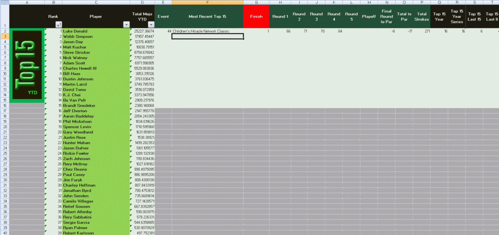
Table in the first image is created from data in the data sheet pictured in the second image. Both tabs are in the same spreadsheet. Each number in the list in column D of the first image is a sum of U in the separate data sheet tab for the particular player (player is C in this sheet, E in the data sheet).

The green and white block areas of the pic below (going down the sheet) are top 15 finishes in PGA golf events (tournaments). Each block contains 15 names and associated tournament data. This is the data entry area of the data sheet. Most of this is hidden, because it is not related to the problem. To the right is generated data. The farthest right columns, X and Y, are running sums of the number found in U (a tournament specific generated number). They are calculated using only data from the previous 15 golf tournaments (120) entries overall), in the case of X (Mojo Last 8), and only the previous 225 entries, in the case of Y (Mojo Last 15). Then the current event is added in for a total of 16 events. The total span is 135 rows for the X data and 240 rows for the Y data.

The latest entry of X and of Y are the highest for their respective ranges. I need to create a table like in image one, which contains each player (column E of the data sheet) represented in the range of the bottom 135 entries of the data sheet, each player listed one time (Formula 1 needed). The list will be placed in C2 of tab 2 (see below for tab names). Then I need a formula to return the sum of the U column data in the data sheet (image 2) over the 135 lines from the bottom of the column for each specific player represented in that range (the ones in the player list for the range created by formula 1). The number is already there in the data sheet in the X column, so what I think would be best would be to create the list of players in the range (this would be the first column of the list and placed in C2 down of tab 2). Then find the latest X for each player in the list in the range of the bottom 135 and return that number for each player represented to the table next to the player's name. I don't know how to do this, and I am having no luck. The database of data shown in pic 2 gets larger throughout the year with the addition of each tournament, so I cannot set specific ranges for the last 135 for the table. I just either have to find the last X in the datasheet over the last 135 rows for each player or sum up for the player from the bottom his U column entries over the last 135 rows.
Here is the formula for the data in the table in picture 1. The span here for calculating the number was the whole spreadsheet of data in the data sheet, 18-962. The players' names are all the players represented in the range. It sums U for each E and returns the total (to column D in image 1) next to the player's name (column C in image 1) in sheet 4:
=SUMIF(DataSheet!E$18:E$962,C2,DataSheet!U$18:U$962)
Basically, I need something similar but that either:
1. Sums the Us for the bottom 135 lines of the U column in the data sheet (pic 2) for each player
or
2. Returns the first column X value in the data sheet (pic 2) for each player from the bottom over the bottom 135 lines. The result will be compiled in tab 2.
Data Sheet is called: DataSheet
tab 4 is called: Top 15ers YTD
tab 2 is called: Top 15 Last 8
Spreadsheet is called: mojo_masters_2(1)
I am beside myself about this, so I would love any help whatsoever. Thankyou!
Table in the first image is created from data in the data sheet pictured in the second image. Both tabs are in the same spreadsheet. Each number in the list in column D of the first image is a sum of U in the separate data sheet tab for the particular player (player is C in this sheet, E in the data sheet).

The green and white block areas of the pic below (going down the sheet) are top 15 finishes in PGA golf events (tournaments). Each block contains 15 names and associated tournament data. This is the data entry area of the data sheet. Most of this is hidden, because it is not related to the problem. To the right is generated data. The farthest right columns, X and Y, are running sums of the number found in U (a tournament specific generated number). They are calculated using only data from the previous 15 golf tournaments (120) entries overall), in the case of X (Mojo Last 8), and only the previous 225 entries, in the case of Y (Mojo Last 15). Then the current event is added in for a total of 16 events. The total span is 135 rows for the X data and 240 rows for the Y data.

The latest entry of X and of Y are the highest for their respective ranges. I need to create a table like in image one, which contains each player (column E of the data sheet) represented in the range of the bottom 135 entries of the data sheet, each player listed one time (Formula 1 needed). The list will be placed in C2 of tab 2 (see below for tab names). Then I need a formula to return the sum of the U column data in the data sheet (image 2) over the 135 lines from the bottom of the column for each specific player represented in that range (the ones in the player list for the range created by formula 1). The number is already there in the data sheet in the X column, so what I think would be best would be to create the list of players in the range (this would be the first column of the list and placed in C2 down of tab 2). Then find the latest X for each player in the list in the range of the bottom 135 and return that number for each player represented to the table next to the player's name. I don't know how to do this, and I am having no luck. The database of data shown in pic 2 gets larger throughout the year with the addition of each tournament, so I cannot set specific ranges for the last 135 for the table. I just either have to find the last X in the datasheet over the last 135 rows for each player or sum up for the player from the bottom his U column entries over the last 135 rows.
Here is the formula for the data in the table in picture 1. The span here for calculating the number was the whole spreadsheet of data in the data sheet, 18-962. The players' names are all the players represented in the range. It sums U for each E and returns the total (to column D in image 1) next to the player's name (column C in image 1) in sheet 4:
=SUMIF(DataSheet!E$18:E$962,C2,DataSheet!U$18:U$962)
Basically, I need something similar but that either:
1. Sums the Us for the bottom 135 lines of the U column in the data sheet (pic 2) for each player
or
2. Returns the first column X value in the data sheet (pic 2) for each player from the bottom over the bottom 135 lines. The result will be compiled in tab 2.
Data Sheet is called: DataSheet
tab 4 is called: Top 15ers YTD
tab 2 is called: Top 15 Last 8
Spreadsheet is called: mojo_masters_2(1)
I am beside myself about this, so I would love any help whatsoever. Thankyou!


