Tab Reference in Formula

fivanaj

New Member
Joined
Jun 21, 2021
Messages
3
Office Version
  1. 365
Platform
  1. Windows
Hello Excel Experts,

I need some help (if possible) regarding formulas that contain a tab reference. Specifically, I am trying to find out if I can incorporate a formula that based off of a text contained in the same cell on every sheet, that it would change which tab will be referenced. In the screenshot below, you will see I underlined in red a specific tab being referenced to in an external workbook. What I am trying to do is have this "PL07" portion be a reference to the "PL07" in cell B2.

Any help would be greatly appreciated.

1677103838729.png
 

Attachments

  • 1677103822210.png
    1677103822210.png
    33.4 KB · Views: 6

Excel Facts

What do {} around a formula in the formula bar mean?
{Formula} means the formula was entered using Ctrl+Shift+Enter signifying an old-style array formula.
you can add an Indirect
bit difficult to see an image and redu the formulas and setup

but here is a simplified version
=INDEX(INDIRECT("'"&Sheet1!B2&"'!$B$1:$B$10"),MATCH(Sheet1!A4,INDIRECT("'"&Sheet1!B2&"'!$A$1:$A$10"),0))

Where I have a sheet1 with this formula on
A sheet named PLO7

in B2 on sheet 1 - i put PLO7
then in the formula we use INDIRECT() to refence the contents of a cell , in this case B2 and use the content PLO7 within a formula

Book3
AB
1
2plo7
3
4csheet plo7 - a3
Sheet1
Cell Formulas
RangeFormula
B4B4=INDEX(INDIRECT("'"&Sheet1!B2&"'!$B$1:$B$10"),MATCH(Sheet1!A4,INDIRECT("'"&Sheet1!B2&"'!$A$1:$A$10"),0))


Book3
AB
1asheet plo7 - a1
2bsheet plo7 - a2
3csheet plo7 - a3
4dsheet plo7 - a4
5esheet plo7 - a5
6fsheet plo7 - a6
7gsheet plo7 - a7
plo7


Note: Images are difficult to see , and also requires that I input all the data myself, which means I may make an error, which is very time consuming, and from my point of view less likely to get a response, if a complicated spreadsheet. Plus we cannot see any of the formulas used.

Therefore -

A SMALL sample spreadsheet, around 10-20 rows, would help a lot here, with all sensitive data removed, and expected results mocked up and manually entered, with a few notes of explanation.

MrExcel has a tool called “XL2BB” that lets you post samples of your data and will allow us to copy/paste your sample data into our Excel spreadsheets, saving a lot of time.

You can also test to see if it works ok, in the "Test Here" forum.

OR if you cannot get XL2BB to work, or have restrictions on your PC , then put the sample spreadsheet onto a share
I only tend to goto OneDrive, Dropbox or google docs , as I'm never certain of other random share sites and possible virus.
Please make sure you have a representative data sample and also that the data has been desensitised, remember this site is open to anyone with internet access to see - so any sensitive / personal data should be removed
 
Upvote 0
Hi & welcome to MrExcel.
If the external workbook is closed then it cannot be done, but if the workbook is open you can use Indirect as shown by etaf.
 
Upvote 0
Hi & welcome to MrExcel.
If the external workbook is closed then it cannot be done, but if the workbook is open you can use Indirect as shown by etaf.
Financial Flash - 2023.02.16 FEB WK2 change.xlsm
ABCDEFGIJLMOPRSUVXYZADAFAGAHAIAJAKALAM
1Feb-23
2PL07Select Status ------->IncompleteIncompleteIncompleteIncompleteIncompleteIncompleteNote: MUST have comments for any/all PERFORMANCE variances that round to +/- $0.1M
3FEBRUARY01+11%WK1WK2WK3WK4WD2WD7MTDVARIANCE B/(W)VOL.MIXF/XECON.PERF.COMMENTS (required if yellow - automatically highlighted)
4
5Days in Month28(28)
6Holidays--
7Weekdays (M-F)20(20)
8Saturdays4(4)
9Sundays4(4)
10Weekend Days8(8)
11Weekends Days & Holidays8(8)
12Sundays & Holidays (Double-Time)4(4)
13
14EDI Tracking-
15Past Due Tracking-
16
17Gross Sales6,210100.0%(6,210)(6,210)
18Past Due-0.0%--
19S&D Adjustments-0.0%--
20NCP/Pricing-0.0%---
21TOTAL SALES6,210100.0%------(6,210)(6,210)----
22SALESTRUEOKOKOKOKOKOK
23STD Material4,81377.5%4,8134,813-
24Value Add -0.0%---
25Copper-0.0%---
26Precious Metals-0.0%---
27Resin(460)-7.4%(460)(460)-Positive PPV on PBT & Nylon
28POV (MCIP Design) - booked-0.0%---
29PPV (MCIP P2P) - booked-0.0%---
30POV (MCIP Design) - fcst-0.0%---
31PPV (MCIP P2P) - fcst-0.0%---
32POV (MCIP Design) - pipeline-0.0%---
33PPV (MCIP P2P) - pipeline-0.0%---
34Rebates-0.0%---
35Material Other00.0%00-
36SUBTOTAL MATERIAL4,35370.1%------4,3534,353----
37MATERIALTRUEOKOKOKOKOKOK
PL07
Cell Formulas
RangeFormula
B1B1=DATEVALUE($B$3&" 1, "&HOLIDAYS!$AA$1)
B2B2=RIGHT(CELL("filename",A1),LEN(CELL("filename",A1))-SEARCH("]",CELL("filename",A1)))
B3B3='TOTAL NA'!$B$3
D3D3=UNIQUE('TOTAL NA'!$D$3)
S3S3='TOTAL NA'!$O$3
V3V3='TOTAL NA'!$Q$3
D5D5=DAY(EOMONTH(B1,0))
D6D6=COUNTIFS(HOLIDAYS!$AA$3:$AA$18,">="&B1,HOLIDAYS!$AA$3:$AA$18,"<"& EDATE(B1,1))
D7D7=NETWORKDAYS(B1,EOMONTH(B1,0))
D8D8=DAY(EOMONTH(B1,0))-NETWORKDAYS.INTL(B1,EOMONTH(B1,0),17)
D9D9=DAY(EOMONTH(B1,0))-NETWORKDAYS.INTL(B1,EOMONTH(B1,0),11)
D10D10=SUM(D8:D9)
D11D11=SUM(D6,D10)
D12D12=SUM(D6,D9)
AD5:AD12,AD17:AD20,AD14:AD15AD5=IFERROR(AA5-D5,0)
AD21,D21,V21,S21,P21,M21,J21,G21,AG21:AK21AD21=SUM(AD17:AD20)
AG17:AG20AG17=IFERROR(AD17-AK17-AJ17-AI17,"")
AK20AK20=AD20
E17:E21,E23:E36E17=IFERROR(D17/D$21,"")
G22,S37,P37,M37,J37,G37,S22,P22,M22,J22G22=IF(J$2="Complete","OK",IF(G$2="Complete",G21=$AA21,"OK"))
V22,V37V22=IF(V$2="Complete",V21=$AA21,"OK")
AD23:AD35AD23=IFERROR(D23-AA23,0)
AD36,V36,D36,AG36:AK36,S36,P36,M36,J36,G36AD36=SUM(AD23:AD35)
AG23:AG35AG23=IFERROR(-AG$21*E23,"")
AK23:AK35AK23=AD23-SUM(AG23:AJ23)
D17:D20,D23:D35D17=INDEX('W:\p\USOHWAR\NABF_2011\NA DCS\2023\01+11 Forecast\Forecast Review\[CS NA 2023 1+11 Final by Plant_V2.xlsx]PL07'!$C:$Y,MATCH(B17,'W:\p\USOHWAR\NABF_2011\NA DCS\2023\01+11 Forecast\Forecast Review\[CS NA 2023 1+11 Final by Plant_V2.xlsx]PL07'!$B:$B,0),VLOOKUP(LEFT($B$3,3),STATUS!$E$52:$G$63,3,FALSE))
D22,D37D22=D21=INDEX('W:\p\USOHWAR\NABF_2011\NA DCS\2023\01+11 Forecast\Forecast Review\[CS NA 2023 1+11 Final by Plant_V2.xlsx]PL07'!$C:$Y,MATCH(B22,'W:\p\USOHWAR\NABF_2011\NA DCS\2023\01+11 Forecast\Forecast Review\[CS NA 2023 1+11 Final by Plant_V2.xlsx]PL07'!$B:$B,0),VLOOKUP(LEFT($B$3,3),STATUS!$E$52:$G$63,3,FALSE))
Cells with Conditional Formatting
CellConditionCell FormatStop If True
AM12Expression=$AD12>49.99textNO
AM12Expression=$AD12<-49.99textNO
AG12:AK12Cell Value>49.99textNO
AG12:AK12Cell Value<-49.99textNO
AG12:AK12Other TypeIcon setNO
AD12Other TypeIcon setNO
AM11Expression=$AD11>49.99textNO
AM11Expression=$AD11<-49.99textNO
AG11:AK11Cell Value>49.99textNO
AG11:AK11Cell Value<-49.99textNO
AG11:AK11Other TypeIcon setNO
AD11Other TypeIcon setNO
AM7Expression=$AD7>49.99textNO
AM7Expression=$AD7<-49.99textNO
AG7:AK7Cell Value>49.99textNO
AG7:AK7Cell Value<-49.99textNO
AG7:AK7Other TypeIcon setNO
AD7Other TypeIcon setNO
AM10Expression=$AD10>49.99textNO
AM10Expression=$AD10<-49.99textNO
AG10:AK10Cell Value>49.99textNO
AG10:AK10Cell Value<-49.99textNO
AG10:AK10Other TypeIcon setNO
AD10Other TypeIcon setNO
AM8Expression=$AD8>49.99textNO
AM8Expression=$AD8<-49.99textNO
AG8:AK8Cell Value>49.99textNO
AG8:AK8Cell Value<-49.99textNO
AG8:AK8Other TypeIcon setNO
AD8Other TypeIcon setNO
AG6:AK6Cell Value>49.99textNO
AG6:AK6Cell Value<-49.99textNO
AG6:AK6Other TypeIcon setNO
AD6Other TypeIcon setNO
AG5:AK6Cell Value>49.99textNO
AG5:AK6Cell Value<-49.99textNO
AG5:AK5Other TypeIcon setNO
AD5Other TypeIcon setNO
AM9,AM14:AM15Expression=$AD9>49.99textNO
AM9,AM14:AM15Expression=$AD9<-49.99textNO
AG9:AK9Cell Value>49.99textNO
AG9:AK9Cell Value<-49.99textNO
AG9:AK9Other TypeIcon setNO
AG15:AK15Cell Value>49.99textNO
AG15:AK15Cell Value<-49.99textNO
AG15:AK15Other TypeIcon setNO
AD15Other TypeIcon setNO
AG14:AK14Cell Value>49.99textNO
AG14:AK14Cell Value<-49.99textNO
AG14:AK14Other TypeIcon setNO
AD9Other TypeIcon setNO
AD9,AD14Other TypeIcon setNO
G2Cell Value="Complete"textNO
G2Cell Value="Incomplete"textNO
J2Cell Value="Complete"textNO
J2Cell Value="Incomplete"textNO
M2Cell Value="Complete"textNO
M2Cell Value="Incomplete"textNO
P2Cell Value="Complete"textNO
P2Cell Value="Incomplete"textNO
S2Cell Value="Complete"textNO
S2Cell Value="Incomplete"textNO
V2Cell Value="Complete"textNO
V2Cell Value="Incomplete"textNO
G37:H37,J37:K37,M37:N37,P37:Q37,S37:T37,V37Cell Value="OK"textNO
G37:H37,J37:K37,M37:N37,P37:Q37,S37:T37,V37Cell Value=FALSEtextNO
G37:H37,J37:K37,M37:N37,P37:Q37,S37:T37,V37Cell Value=TRUEtextNO
G22:H22,J22:K22,M22:N22,P22:Q22,S22:T22,V22Cell Value="OK"textNO
G22:H22,J22:K22,M22:N22,P22:Q22,S22:T22,V22Cell Value=FALSEtextNO
G22:H22,J22:K22,M22:N22,P22:Q22,S22:T22,V22Cell Value=TRUEtextNO
AM17:AM20,AM5:AM6Expression=$AD5>49.99textNO
AM17:AM20,AM5:AM6Expression=$AD5<-49.99textNO
AK23:AK35,AK38:AK43,AK48:AK70,AK76,AK81:AK89,AK17:AK20Cell Value>49.99textNO
AK23:AK35,AK38:AK43,AK48:AK70,AK76,AK81:AK89,AK17:AK20Cell Value<-49.99textNO
AK38:AK43,AK46,AK48:AK70,AK73,AK75:AK77,AK79,AK81:AK90,AK23:AK36,AK17:AK21Other TypeIcon setNO
AM23:AM35Expression=$AK23>49.99textNO
AM23:AM35Expression=$AK23<-49.99textNO
D37Cell Value=FALSEtextNO
D37Cell Value=TRUEtextNO
D22Cell Value=FALSEtextNO
D22Cell Value=TRUEtextNO
AD17:AD21,AD23:AD36,AD38:AD43,AD46,AD48:AD70,AD73,AD75:AD77,AD79,AD81:AD90Other TypeIcon setNO
AD17:AD20Other TypeIcon setNO
Cells with Data Validation
CellAllowCriteria
P2ListIncomplete, Complete
J2ListIncomplete, Complete
S2ListIncomplete, Complete
M2ListIncomplete, Complete
V2ListIncomplete, Complete
G2ListIncomplete, Complete
 
Upvote 0
on this occasion not , as you have reference to other sheets and other workbooks

BUT
it does at least allow the formula to be edited

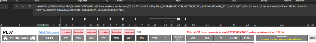
is this the formula IN D17 you want to refer to B2 to get the sheet name

=INDEX('W:\p\USOHWAR\NABF_2011\NA DCS\2023\01+11 Forecast\Forecast Review\[CS NA 2023 1+11 Final by Plant_V2.xlsx]PL07'!$C:$Y,MATCH(B17,'W:\p\USOHWAR\NABF_2011\NA DCS\2023\01+11 Forecast\Forecast Review\[CS NA 2023 1+11 Final by Plant_V2.xlsx]PL07'!$B:$B,0),VLOOKUP(LEFT($B$3,3),STATUS!$E$52:$G$63,3,FALSE))

And this one in D22
=D21=INDEX('W:\p\USOHWAR\NABF_2011\NA DCS\2023\01+11 Forecast\Forecast Review\[CS NA 2023 1+11 Final by Plant_V2.xlsx]PL07'!$C:$Y,MATCH(B22,'W:\p\USOHWAR\NABF_2011\NA DCS\2023\01+11 Forecast\Forecast Review\[CS NA 2023 1+11 Final by Plant_V2.xlsx]PL07'!$B:$B,0),VLOOKUP(LEFT($B$3,3),STATUS!$E$52:$G$63,3,FALSE))

As fluff said
If the external workbook is closed then it cannot be done,

So is the reference work book - closed ?

=INDEX('W:\p\USOHWAR\NABF_2011\NA DCS\2023\01+11 Forecast\Forecast Review\[CS NA 2023 1+11 Final by Plant_V2.xlsx]PL07'!$C:$Y,MATCH(B17,'W:\p\USOHWAR\NABF_2011\NA DCS\2023\01+11 Forecast\Forecast Review\[CS NA 2023 1+11 Final by Plant_V2.xlsx]PL07'!$B:$B,0),VLOOKUP(LEFT($B$3,3),STATUS!$E$52:$G$63,3,FALSE))

using my example
=INDEX(INDIRECT("'"&Sheet1!B2&"'!$B$1:$B$10"),MATCH(Sheet1!A4,INDIRECT("'"&Sheet1!B2&"'!$A$1:$A$10"),0))

to change you info

INDIRECT("'W:\p\USOHWAR\NABF_2011\NA DCS\2023\01+11 Forecast\Forecast Review\[CS NA 2023 1+11 Final by Plant_V2.xlsx]"&B2&"'!$C:$Y")

BUT notice the whole path and range is in "" so will not change if you copy the formula to different cells

MATCH(B17,indirect("'W:\p\USOHWAR\NABF_2011\NA DCS\2023\01+11 Forecast\Forecast Review\[CS NA 2023 1+11 Final by Plant_V2.xlsx]"&B2&"'!$B:$B")


so to change this formula
=INDEX('W:\p\USOHWAR\NABF_2011\NA DCS\2023\01+11 Forecast\Forecast Review\[CS NA 2023 1+11 Final by Plant_V2.xlsx]PL07'!$C:$Y,MATCH(B17,'W:\p\USOHWAR\NABF_2011\NA DCS\2023\01+11 Forecast\Forecast Review\[CS NA 2023 1+11 Final by Plant_V2.xlsx]PL07'!$B:$B,0),VLOOKUP(LEFT($B$3,3),STATUS!$E$52:$G$63,3,FALSE))

TO
=INDEX(
INDIRECT("'W:\p\USOHWAR\NABF_2011\NA DCS\2023\01+11 Forecast\Forecast Review\[CS NA 2023 1+11 Final by Plant_V2.xlsx]"&B2&"'!$C:$Y"),
MATCH(B17,indirect("'W:\p\USOHWAR\NABF_2011\NA DCS\2023\01+11 Forecast\Forecast Review\[CS NA 2023 1+11 Final by Plant_V2.xlsx]"&B2&"'!$B:$B"),0),
VLOOKUP(LEFT($B$3,3),STATUS!$E$52:$G$63,3,FALSE))
 
Upvote 0

Forum statistics

Threads
1,214,589
Messages
6,120,415
Members
448,960
Latest member
AKSMITH

We've detected that you are using an adblocker.

We have a great community of people providing Excel help here, but the hosting costs are enormous. You can help keep this site running by allowing ads on MrExcel.com.
Allow Ads at MrExcel

Which adblocker are you using?

Disable AdBlock

Follow these easy steps to disable AdBlock

1)Click on the icon in the browser’s toolbar.
2)Click on the icon in the browser’s toolbar.
2)Click on the "Pause on this site" option.
Go back

Disable AdBlock Plus

Follow these easy steps to disable AdBlock Plus

1)Click on the icon in the browser’s toolbar.
2)Click on the toggle to disable it for "mrexcel.com".
Go back

Disable uBlock Origin

Follow these easy steps to disable uBlock Origin

1)Click on the icon in the browser’s toolbar.
2)Click on the "Power" button.
3)Click on the "Refresh" button.
Go back

Disable uBlock

Follow these easy steps to disable uBlock

1)Click on the icon in the browser’s toolbar.
2)Click on the "Power" button.
3)Click on the "Refresh" button.
Go back
Back
Top