Time Formula

[JumboCactuar]

Hi,
if i have the following in the format below:

Shift Times:
08:00-17:00
08:00-17:00
08:00-17:00
08:00-17:00
08:00-17:00
08:30-17:30
08:30-17:30
08:30-17:30
08:30-17:30
08:30-17:30
09:00-18:00
09:30-18:30
10:00-19:00

Hour - answers in red which i need formula for (Total hours from available users - example hour 08 - 5 users start at 08:00 = 5 hours plus 5 start at 08:30 = 2.5)
08 - 7.5
09 - 12
10 - 13

Ones who start 08:00 and 08:30 are added to 09:00 as its within their hours

Thanks for any help, i know this looks confusing. I think im best to start converting these into numeric values like 08:00 = 80000 and 08:30 = 80500

 

[inactiveuserps07]

Re: Need help with Time Formula please

@JumboCactuar, first, it seems to me that your 09 figure should be 11.5, not 12 (i.e., 11 people fully on by 9:00 and then add 0.5 for the person who came on at 9:30).

That said, assuming that your Shift Times header is in A1 with the shifts in A2:A14, and assuming your hourly list (08 - 19) begins in C2, the following array "mega-formula" (confirmed with Ctrl+Shift+Enter) in D2 and drag-copied down should work:

=SUM(IF(VALUE(LEFT(A$2:A$14,2))<C2,IF((TIMEVALUE(MID(A$2:A$14,FIND("-",A$2:A$14)+1,10))*24)>C2,1,0),0))+SUM(IF(VALUE(LEFT(A$2:A$14,2))=C2,IF(VALUE(MID(A$2:A$14,4,2))=0,IF((TIMEVALUE(MID(A$2:A$14,FIND("-",A$2:A$14)+1,10))*24)>C2,1,0),0),0))+SUM(IF(VALUE(LEFT(A$2:A$14,2))=C2,IF(VALUE(MID(A$2:A$14,4,2))=30,IF((TIMEVALUE(MID(A$2:A$14,FIND("-",A$2:A$14)+1,10))*24)>C2,0.5,0),0),0))

 

[JumboCactuar]

Re: Need help with Time Formula please

@JumboCactuar, first, it seems to me that your 09 figure should be 11.5, not 12 (i.e., 11 people fully on by 9:00 and then add 0.5 for the person who came on at 9:30).

That said, assuming that your Shift Times header is in A1 with the shifts in A2:A14, and assuming your hourly list (08 - 19) begins in C2, the following array "mega-formula" (confirmed with Ctrl+Shift+Enter) in D2 and drag-copied down should work:

=SUM(IF(VALUE(LEFT(A$2:A$14,2))<c2,if((timevalue(mid(a$2:a$14,find("-",a$2:a$14)+1,10))*24)>C2,1,0),0))+SUM(IF(VALUE(LEFT(A$2:A$14,2))=C2,IF(VALUE(MID(A$2:A$14,4,2))=0,IF((TIMEVALUE(MID(A$2:A$14,FIND("-",A$2:A$14)+1,10))*24)>C2,1,0),0),0))+SUM(IF(VALUE(LEFT(A$2:A$14,2))=C2,IF(VALUE(MID(A$2:A$14,4,2))=30,IF((TIMEVALUE(MID(A$2:A$14,FIND("-",A$2:A$14)+1,10))*24)>C2,0.5,0),0),0))

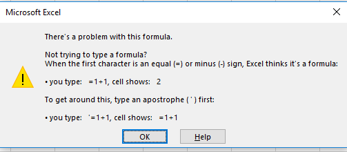
thanks for the reply, i tried this but it throws an error:

after error the first C2 in the formula is highlighted, maybe an error there? =SUM(IF(VALUE(LEFT(A$2:A$14,2))<c2,if((timevalue(mid(a$2:a$14,find("-",a$2:a$14)+1,10))*24) style="color: rgb(51, 51, 51); font-size: 12px;">C2,1,0)</c2,if((timevalue(mid(a$2:a$14,find("-",a$2:a$14)+1,10))*24)>

put the shift times in A2 downwards
and hours 06 onwards in C2</c2,if((timevalue(mid(a$2:a$14,find("-",a$2:a$14)+1,10))*24)>

 

[inactiveuserps07]

Re: Need help with Time Formula please

@JumboCactuar, yes, somehow a less-than sign got cut from that formula when I pasted it:

=SUM(IF(VALUE(LEFT(A$2:A$14,2))[B][COLOR=#0000ff]<[/COLOR][/B]<c2,if((timevalue(mid(a$2:a$14,find("-",a$2:a$14)+1,10))*24)>C2,1,0),0))+SUM(IF(VALUE(LEFT(A$2:A$14,2))=C2,IF(VALUE(MID(A$2:A$14,4,2))=0,IF((TIMEVALUE(MID(A$2:A$14,FIND("-",A$2:A$14)+1,10))*24)>C2,1,0),0),0))+SUM(IF(VALUE(LEFT(A$2:A$14,2))=C2,IF(VALUE(MID(A$2:A$14,4,2))=30,IF((TIMEVALUE(MID(A$2:A$14,FIND("-",A$2:A$14)+1,10))*24)>C2,0.5,0),0),0))</c2,if((timevalue(mid(a$2:a$14,find("-",a$2:a$14)+1,10))*24)>

 

[JumboCactuar]

Re: Need help with Time Formula please

@JumboCactuar, yes, somehow a less-than sign got cut from that formula when I pasted it:

=SUM(IF(VALUE(LEFT(A$2:A$14,2))[B][COLOR=#0000ff]<[/COLOR][/B]<c2,if((timevalue(mid(a$2:a$14,find("-",a$2:a$14)+1,10))*24)>C2,1,0),0))+SUM(IF(VALUE(LEFT(A$2:A$14,2))=C2,IF(VALUE(MID(A$2:A$14,4,2))=0,IF((TIMEVALUE(MID(A$2:A$14,FIND("-",A$2:A$14)+1,10))*24)>C2,1,0),0),0))+SUM(IF(VALUE(LEFT(A$2:A$14,2))=C2,IF(VALUE(MID(A$2:A$14,4,2))=30,IF((TIMEVALUE(MID(A$2:A$14,FIND("-",A$2:A$14)+1,10))*24)>C2,0.5,0),0),0))</c2,if((timevalue(mid(a$2:a$14,find("-",a$2:a$14)+1,10))*24)>

same error but now at this stage:
=SUM(IF(VALUE(LEFT(A$2:A$14,2))<C2,1,0),0))

 

[inactiveuserps07]

Re: Need help with Time Formula please

And if your shift times will always look exactly as they do, you can shorten it a bit to this:

[COLOR=#333333]=SUM(IF(VALUE(LEFT(A$2:A$14,2))[/COLOR][B]<[/B]<c2,if((timevalue(mid(a$2:a$14,find("-",a$2:a$14)+1,10))*24) style="color: rgb(51, 51, 51); font-size: 12px;">C2,1,0),0))+SUM(IF(VALUE(LEFT(A$2:A$14,2))=C2,IF(VALUE(MID(A$2:A$14,4,2))=0,IF((TIMEVALUE(MID(A$2:A$14,7,10))*24)>C2,1,0),0),0))+SUM(IF(VALUE(LEFT(A$2:A$14,2))=C2,IF(VALUE(MID(A$2:A$14,4,2))=30,IF((TIMEVALUE(MID(A$2:A$14,7,10))*24)>C2,0.5,0),0),0))</c2,if((timevalue(mid(a$2:a$14,find("-",a$2:a$14)+1,10))*24)>

 

[wideboydixon]

Re: Need help with Time Formula please

How about this:

Book1
	A	B	C	D
1	Shift Times:		Hour	Available
2	08:00-17:00		08	7.5
3	08:00-17:00		09	11.5
4	08:00-17:00		10	13
5	08:00-17:00
6	08:00-17:00
7	08:30-17:30
8	08:30-17:30
9	08:30-17:30
10	08:30-17:30
11	08:30-17:30
12	09:00-18:00
13	09:30-18:30
14	10:00-19:00
Sheet1

Cell Formulas
Range	Formula
D2	=COUNTIF($A$2:$A$114,"<="&TEXT(TIME($C2,0,0),"hh:mm")&"-9")+COUNTIF($A$2:$A$114,TEXT(TIME($C2,30,0),"hh:mm")&"*")/2

WBD

 

[inactiveuserps07]

Re: Need help with Time Formula please

@JumboCactuar, as far as I can see, there are no instances where three right parentheses follow that formula portion. Are you remembering to use Ctrl+Shift+Enter after every time you edit?

And my formula is longer than others because you have to account for who goes OFF shift as the hours increase throughout the day.

 

[wideboydixon]

Re: Need help with Time Formula please

Having said that, it won't produce a value of 1.5 for hour 18 which you might want ...

WBD

 

[wideboydixon]

Re: Need help with Time Formula please

Hi @ErikTyler,

The first SUM() in your formula has 4 opening parentheses and 5 closing ones.

WBD