Time stamp using with "if,countif" function...

[madhanji]

Dear Seniors.Excel Masters
i have attach the image for your reference,
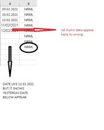
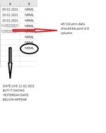
A column should be "today date stamp" when column B has "NRML" string,
so i used IF condition

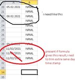
IF(B20="","",IF(B20="NRML",now(),"HI"))

it's working fine..
but while drag-down the formula time stamps shows A column but i dont need it..
first date is only ok for entire day...
means as per attached picture
so i tried countif function but not succeed as per my knowledge..
please help...

Thanks in advance..

 

[jasonb75]

Best guess based on the information provided, I've assumed that the first Date stamp (a Time stamp has time as well as date) will be in A2 and the first "NRML" in B2.

This is only possible with circular references, so it needs to be set up properly or it will not work.

Note that you need to go to Formulas tab of your Excel options and check the box to 'Enable iterative calculations' before entering the formulas.
Also, you must clear any existing "NRML" entries from column B before entering the formulas.

If you do not follow the steps above then this will not work.

Formula to enter into A2 and fill down,

=IF(B2="NRML",IF(A2<>"",A2,IF(COUNTIF(A$1:A1,TODAY()),"",TODAY())),"")

 

[madhanji]

Dear Jasonb75,Thanks for prompt reply and solution,
S,it.'s working well ...even will check tomorrow and revert you sir..

Happy life.

 

[madhanji]

HII DEAR JASONB75,

=IF(B2="NRML",IF(A2<>"",A2,IF(COUNTIF(A$1:A1,TODAY()),"",TODAY())),"")

above your formula works yesterday nly, today it shows wrong means exact/required output not get...please see attached picture for your reference ..

Please help to resolve it sir..

Happy life.

 

[madhanji]

Dear seniors /Excel Masters..
please look into my request of post no1 ,jasonb75 provided half solution in post no2, but not succeeded .please..

Happy Life

 

[jasonb75]

As far as I can see, the solution that I provided is correct for what you have asked for.

I can not understand what you are trying to say is wrong with it.

 

[madhanji]

Dear Jasonb75 sir,please look into post no:4/attached picture here sir,i indicate the error in attached picture..
even please see in my post no 1 attached picture , i noticed extra date in same day should be trim sir..
but your formula gives extra date in same day removed ,its well, next day in B COLUMN "NRML" entered A COLUMN date appear below the yesterday date instead of today NRML corresponding A column
i noticed error in attached picture here.

hope maybe i explain correctly...

Happy life







;

 

[jasonb75]

The image in post 1 shows the last 2 dates for 11/02/2021 crossed out with a red line which indicates that the date should be next to the first "NRML" entered on that date.

In your latest image it appears that you want the date to be next to the last "NRML" for the day instead of the first. Is this correct?

 

[madhanji]

The image in post 1 shows the last 2 dates for 11/02/2021 crossed out with a red line which indicates that the date should be next to the first "NRML" entered on that date.

the crossed red line of extra date on same day no need, so should be trim.

In your latest image it appears that you want the date to be next to the last "NRML" for the day instead of the first. Is this correct?

s sir. now you catch up my point..
please give me a solution...

 

[jasonb75]

Change the formula to

=IF(B2="NRML",IF(A2<>"",A2,TODAY()),"")

Then use conditional formatting to change the font colour to white in the rows where the date is not needed.

Select A2:A100, then go to conditional formatting.
Create a new rule, using a formula. The formula to use will be

=A2=A1

Set the font colour and click OK / Apply as applicable to finish setting the rule.