To loop through rows and columns to divide and vlookup

Ann Ooi

New Member
Joined
Jun 12, 2020
Messages
40
Office Version
  1. 365
Platform
  1. Windows
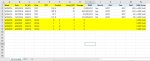
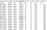
I have sheet "DataCompile" which I have columns I to L that I would like to vlookup data from sheet "WW", the data are compile from week to week, so I need to vlookup the new lines added ( as picture shown rows 6 to 9). And at column M, I need to divide G2/E2 for yield calculation, follow by column N, with if formula [=IF(M5<=0.3,"=<30% Yield",IF(M5<=0.6,"=<60% Yield", "60%><=100% Yield"))]. I can manually added this with excel formula, but fail to run it with macro, need helps to rectify the coding as I tried to input for the vlookup and divider, but I failed to insert the IF formula for column N, as the coding totally cannot loop and recognize the cell to insert the value at all, with my coding below.

VBA Code:
Sub UpdateLData()
    
    Application.ScreenUpdating = False
    
   Dim LR As Long
   
    ThisWorkbook.Worksheets("DataCompile").Select
    
    With Sheets("DataCompile").Range("A2", Sheets("DataCompile").Cells(Rows.Count, "A").End(xlUp))
        .Offset(, 8).Formula = "=VLOOKUP(B" & .Row & ",'WD_WW'!$A:$H,4,FALSE)"
        .Offset(, 8).Value = .Offset(, 8).Value
    End With

    With Sheets("DataCompile").Range("A2", Sheets("DataCompile").Cells(Rows.Count, "A").End(xlUp))
        .Offset(, 9).Formula = "=VLOOKUP(B" & .Row & ",'WD_WW'!$C:$F,5,FALSE)"
        .Offset(, 9).Value = .Offset(, 9).Value
    End With

    With Sheets("DataCompile").Range("A2", Sheets("DataCompile").Cells(Rows.Count, "A").End(xlUp))
        .Offset(, 10).Formula = "=VLOOKUP(B" & .Row & ",'WD_WW'!$C:$F,7,FALSE)"
        .Offset(, 10).Value = .Offset(, 10).Value
    End With
    
    With Sheets("DataCompile").Range("A2", Sheets("DataCompile").Cells(Rows.Count, "A").End(xlUp))
        .Offset(, 11).Formula = "=VLOOKUP(B" & .Row & ",'WD_WW'!$C:$F,8,FALSE)"
        .Offset(, 11).Value = .Offset(, 11).Value
    End With
        
    With Sheets("DataCompile").Range("A2", Sheets("DataCompile").Cells(Rows.Count, "A").End(xlUp))
        .Offset(, 12).Formula = "=G2/E2"
        .Offset(, 12).Value = .Offset(, 12).Value

    End With
    
   Range("A1").Select
   
   Application.ScreenUpdating = True
   
   End Sub

And I tried to loop through rows, to add the divider formula, for column M, it's also failed with following coding.

VBA Code:
Sub divide()

Dim max As Long, i As Long, cell As Range, last As Double


last = .Cells(.Rows.Count, "M").End(xlUp).Row
Set cell = Range("M" & last + 1)
max = Range("A" & Rows.Count).End(xlUp).Row

Do
    i = i + 1
    If (cell.Offset(i, 0).Value <> "") Then
        cell.Value = Cells(Rows.Count, "G").Value / Cells(Rows.Count, "E").Value
        Set cell = cell.Offset(i, 0)
        i = 0
    End If
 
    If cell.Row = max Then Exit Sub
Loop
End Sub

Really need help to correct the coding and advise what is the best coding to apply.
 

Attachments

  • Capture1.JPG
    Capture1.JPG
    162.9 KB · Views: 11
  • WW sheet.JPG
    WW sheet.JPG
    155.2 KB · Views: 12

Excel Facts

Which Excel functions can ignore hidden rows?
The SUBTOTAL and AGGREGATE functions ignore hidden rows. AGGREGATE can also exclude error cells and more.
Try this code, I have done the task without using Vlookup. this is because using VBA to write equations to a worksheet and the writing the generated values back to the worksheet is very very slow way of using VBA. IT is much better to load all the data into a variant array and do all the processing of finding the right row and copying the data in memory. You Vlookup wouldn't have worked becuase some of the columns you selected were beyond the range you had selected so I have guessed that the columns you wanted were counting from Column A .
VBA Code:
Sub Fastupdate()
    Application.ScreenUpdating = False
   
   Dim LR As Long
    ' load all the lookup data into a variant array
    With Sheets("WD_WW")
    lastd = .Cells(Rows.Count, "A").End(xlUp).Row
    Datar = Range(.Cells(1, 1), .Cells(lastd, 8))
    End With
 
    ThisWorkbook.Worksheets("DataCompile").Select
   
    lastrow = Cells(Rows.Count, "A").End(xlUp).Row
    inarr = Range(Cells(1, 1), Cells(lastrow, 1))
    ' define output array with blanks
    Range(Cells(1, 9), Cells(lastrow, 15)) = ""
    outarr = Range(Cells(1, 9), Cells(lastrow, 15))
     For i = 2 To lastrow
        For j = 2 To lastd
          If inarr(i, 1) = Datar(j, 1) Then
           ' copy the data to the outut array
            outarr(i, 1) = Datar(j, 4)
            outarr(i, 2) = Datar(j, 5)
            outarr(i, 3) = Datar(j, 7)
            outarr(i, 4) = Datar(j, 8)
            outarr(i, 5) = inarr(i, 7) / inarr(i, 5)
            '=IF(M5<=0.3,"=<30% Yield",IF(M5<=0.6,"=<60% Yield", "60%><=100% Yield"
            outarr(i, 6) = "60%><=100% Yield"
            If outarr(i, 5) < 0.6 Then
             outarr(i, 6) = "=<60% Yield"
            End If
            If outarr(i, 5) < 0.3 Then
             outarr(i, 6) = "=<30% Yield"
            End If
            Exit For
          End If
        Next j
     Next i
    Range(Cells(1, 9), Cells(lastrow, 15)) = outarr
   
End Sub
Note the code is not tested
 
Upvote 0
Hi Offthelip, I think the code deleted all my previous data in columns I to O. I have these data collected from week to week, and new data are until A-H. So, I need to vlookup the new lines with WW/qtr/mth/years vs the date (column B), and add in yield formula to calculate the yield (column M), and define the yield group as above in column N.
 
Upvote 0
Try this modification, it no longer deletes all the data in columns I to O and it only calculates new values for rows after the last data value in column I
The code does all of the calculations ie. dividing column G by column E and putting in the yield group
VBA Code:
Sub Fastupdate()
    Application.ScreenUpdating = False
  
   Dim LR As Long
    ' load all the lookup data into a variant array
    With Sheets("WD_WW")
    lastd = .Cells(Rows.Count, "A").End(xlUp).Row
    Datar = Range(.Cells(1, 1), .Cells(lastd, 8))
    End With
 
    ThisWorkbook.Worksheets("DataCompile").Select
  
        lastrow = Cells(Rows.Count, "A").End(xlUp).Row
    'load column B into Variant array
    inarr = Range(Cells(1, 2), Cells(lastrow, 2))
' find the last row with data in column I
        lasti = Cells(Rows.Count, "I").End(xlUp).Row
'    Range(Cells(1, 9), Cells(lastrow, 15)) = ""
    outarr = Range(Cells(1, 9), Cells(lastrow, 15))
     For i = lasti To lastrow
        For j = 2 To lastd
          If inarr(i, 1) = Datar(j, 1) Then
           ' copy the data to the outut array
            outarr(i, 1) = Datar(j, 4)
            outarr(i, 2) = Datar(j, 5)
            outarr(i, 3) = Datar(j, 7)
            outarr(i, 4) = Datar(j, 8)
            outarr(i, 5) = inarr(i, 7) / inarr(i, 5)
            '=IF(M5<=0.3,"=<30% Yield",IF(M5<=0.6,"=<60% Yield", "60%><=100% Yield"
            outarr(i, 6) = "60%><=100% Yield"
            If outarr(i, 5) < 0.6 Then
             outarr(i, 6) = "=<60% Yield"
            End If
            If outarr(i, 5) < 0.3 Then
             outarr(i, 6) = "=<30% Yield"
            End If
            Exit For
          End If
        Next j
     Next i
    Range(Cells(1, 9), Cells(lastrow, 15)) = outarr
  
End Sub
 
Upvote 0
Try this modification, it no longer deletes all the data in columns I to O and it only calculates new values for rows after the last data value in column I
The code does all of the calculations ie. dividing column G by column E and putting in the yield group
VBA Code:
Sub Fastupdate()
    Application.ScreenUpdating = False
 
   Dim LR As Long
    ' load all the lookup data into a variant array
    With Sheets("WD_WW")
    lastd = .Cells(Rows.Count, "A").End(xlUp).Row
    Datar = Range(.Cells(1, 1), .Cells(lastd, 8))
    End With

    ThisWorkbook.Worksheets("DataCompile").Select
 
        lastrow = Cells(Rows.Count, "A").End(xlUp).Row
    'load column B into Variant array
    inarr = Range(Cells(1, 2), Cells(lastrow, 2))
' find the last row with data in column I
        lasti = Cells(Rows.Count, "I").End(xlUp).Row
'    Range(Cells(1, 9), Cells(lastrow, 15)) = ""
    outarr = Range(Cells(1, 9), Cells(lastrow, 15))
     For i = lasti To lastrow
        For j = 2 To lastd
          If inarr(i, 1) = Datar(j, 1) Then
           ' copy the data to the outut array
            outarr(i, 1) = Datar(j, 4)
            outarr(i, 2) = Datar(j, 5)
            outarr(i, 3) = Datar(j, 7)
            outarr(i, 4) = Datar(j, 8)
            outarr(i, 5) = inarr(i, 7) / inarr(i, 5)
            '=IF(M5<=0.3,"=<30% Yield",IF(M5<=0.6,"=<60% Yield", "60%><=100% Yield"
            outarr(i, 6) = "60%><=100% Yield"
            If outarr(i, 5) < 0.6 Then
             outarr(i, 6) = "=<60% Yield"
            End If
            If outarr(i, 5) < 0.3 Then
             outarr(i, 6) = "=<30% Yield"
            End If
            Exit For
          End If
        Next j
     Next i
    Range(Cells(1, 9), Cells(lastrow, 15)) = outarr
 
End Sub
Hi, Thank you and it works now.
 
Upvote 0

Forum statistics

Threads
1,214,535
Messages
6,120,090
Members
448,944
Latest member
sharmarick

We've detected that you are using an adblocker.

We have a great community of people providing Excel help here, but the hosting costs are enormous. You can help keep this site running by allowing ads on MrExcel.com.
Allow Ads at MrExcel

Which adblocker are you using?

Disable AdBlock

Follow these easy steps to disable AdBlock

1)Click on the icon in the browser’s toolbar.
2)Click on the icon in the browser’s toolbar.
2)Click on the "Pause on this site" option.
Go back

Disable AdBlock Plus

Follow these easy steps to disable AdBlock Plus

1)Click on the icon in the browser’s toolbar.
2)Click on the toggle to disable it for "mrexcel.com".
Go back

Disable uBlock Origin

Follow these easy steps to disable uBlock Origin

1)Click on the icon in the browser’s toolbar.
2)Click on the "Power" button.
3)Click on the "Refresh" button.
Go back

Disable uBlock

Follow these easy steps to disable uBlock

1)Click on the icon in the browser’s toolbar.
2)Click on the "Power" button.
3)Click on the "Refresh" button.
Go back
Back
Top