Transfer table filtered data to new worksheet in respective column, 2nd tab data transferred under last row in respective columns.

[Dave01]

Dropbox - File Deleted - Simplify your life

www.dropbox.com

Hi

The link above is an extract of a larger macro which works really well, however I am stuck on preparing my final report.

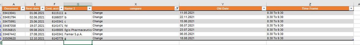
there are a number of tabs which are filtered for change, each tab comparing to the last. In my extract I have two, 09.30 & 12.30, so 12.30 compares to 9.30 to get the change results, works well.

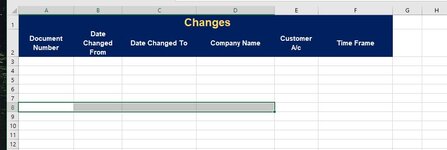
What I am stuck with is transferring these onto another sheet called changes table.

The first transfer works well, although somewhat long winded, I tried many types of VB code, and tried shorting the lines, nothing worked except, individual activate copy and paste.

the second 12.30 tab doesnt cause any errors but doesnt do anything either, it should transfer the visible filtered columns under the last row used of the Changes tables in their respective columns. Im not sure whats happening here, I would be greatful if somebody could take a look. (the tabs use tables)

I tried using this


Set TME = ThisWorkbook.Worksheets("08.30")
'' TME.Range("A:A").Copy Destination:=NDC.Range("A1")
'' TME.Range("E:E").Copy Destination:=NDC.Range("B1")
'' TME.Range("F:F").Copy Destination:=NDC.Range("D1")
'' TME.Range("G:G").Copy Destination:=NDC.Range("C1")
''
instead of all this, but I kept getting errors of paste isnt the same size. Its a bit annoying because there are 7 tabs in total, which will make the program very big.

Sheets("9.30").Activate
Range("A2").Activate
Range(Selection, Selection.End(xlDown)).Copy
Sheets("Changes Table").Activate
Range("A3").Activate
ActiveSheet.Paste

Sheets("9.30").Activate
Range("E2").Activate
Range(Selection, Selection.End(xlDown)).Copy
Sheets("Changes Table").Activate
Range("c3").Activate
ActiveSheet.Paste


Sheets("9.30").Activate
Range("Y2").Activate
Range(Selection, Selection.End(xlDown)).Copy
Sheets("Changes Table").Activate
Range("B3").Activate
ActiveSheet.Paste

Sheets("9.30").Activate
Range("G2").Activate
Range(Selection, Selection.End(xlDown)).Copy
Sheets("Changes Table").Activate
Range("D3").Activate
ActiveSheet.Paste

Sheets("9.30").Activate
Range("F2").Activate
Range(Selection, Selection.End(xlDown)).Copy
Sheets("Changes Table").Activate
Range("E3").Activate
ActiveSheet.Paste


Sheets("9.30").Activate
Range("z2").Activate
Range(Selection, Selection.End(xlDown)).Copy
Sheets("Changes Table").Activate
Range("F3").Activate
ActiveSheet.Paste




Many thanks

Dave.

 

[Fluff]

On the changes tab, select A9 & then hit Ctrl & down arrow. If you keep hitting Ctrl down arrow, you will see that you have loads of data at various points.

Are you always filtering the tables based on "Change" in col E?

 

[Dave01]

Hi fluff,

yes its always column E ( for this test macro) in the main macro (I forgot to unhide columns, so when I copied and pasted it came out as E.

In the main macro its actually X - the condition does change though - its always "change" (it compares change in dates then writes "change"
the visible cells then gets copied to the Changes table, which is really just another separate worksheet.

(all that extra data is probably why my main macro is crashing out),

it just needs to copy visable filtered cells, but I have had every error from Object error, when using the copy visible command to paste cells arnt the same size. (esp when I try to add data to the last row)

thanks for your help,

thanks

dave.

 

[Fluff]

Ok, how about

Sub Dave()
   Dim Ary As Variant, Rws As Variant, Shts As Variant
   Dim i As Long
   
   Shts = Array("9.30", "Table1", "12.30", "Table2")
   For i = 0 To UBound(Shts) Step 2
      With Sheets(Shts(i)).ListObjects(Shts(i + 1))
         Rws = Filter(.Parent.Evaluate(Replace("transpose(if(@=""Change"",row(@)-min(row(@))+1,""^""))", "@", .ListColumns("Compare").DataBodyRange.Address)), "^", False)
         Ary = Application.Index(.DataBodyRange, Application.Transpose(Rws), Array(1, 6, 2, 4, 3, 7))
      End With
      Sheets("Changes Table").Range("A" & Rows.Count).End(xlUp).Offset(1).Resize(UBound(Rws), 6) = Ary
   Next i
End Sub

 

[Dave01]

Hi,

compiled with ought errors, but nothing happened.

I get some of the lines of code




Sheets("Changes Table").Range("A" & Rows.Count).End(xlUp).Offset(1).Resize(UBound(Rws), 6) = Ary - this is addingafter to the last used data

Shts = Array("9.30", "Table1", "12.30", "Table2") - this selects the sheet and the table via name


Rws = Filter(.Parent.Evaluate(Replace("transpose(if(@=""Change"",row(@)-min(row(@))+1,""^""))", "@", .ListColumns("Compare").DataBodyRange.Address)), "^", False)
Ary = Application.Index(.DataBodyRange, Application.Transpose(Rws), Array(1, 6, 2, 4, 3, 7))

not sure about this except the array of columns 1 6 2 4 3 & 7

For i = 0 To UBound(Shts) Step 2
With Sheets(Shts(i)).ListObjects(Shts(i + 1))

this just goes through the tabs where the shts will match the conditions.


thanks

 

[Fluff]

Did you clear all the rubbish below row 8 from the Change sheet first?

 

[Dave01]

In the change tables tab, all data is clear

In the 09.30 data there is data, but I cant remove this from the table as the data is used for someone else, so its just the change filtered I need.

is that what you meant ?

 

[Dave01]

ok I think I see,

I expected it to go from the start of A3, but it looks like its pasting into the start of row A32702, so it works in the correct columns, just way down down down the spreadsheet

 

[Dave01]

Data Selection and Copy

Dim Ary As Variant, Rws As Variant, Shts As Variant
Dim i As Long

Shts = Array("9.30", "Table1", "12.30", "Table2")
For i = 0 To UBound(Shts) Step 2
With Sheets(Shts(i)).ListObjects(Shts(i + 1))
Rws = Filter(.Parent.Evaluate(Replace("transpose(if(@=""Change"",row(@)-min(row(@))+1,""^""))", "@", .ListColumns("Compare").DataBodyRange.Address)), "^", False)
Ary = Application.Index(.DataBodyRange, Application.Transpose(Rws), Array(1, 6, 2, 4, 3, 7))
End With
Sheets("Changes Table").Range("A" & Rows.Count).End(xlUp).Offset(1).Resize(UBound(Rws), 6) = Ary
Next i

Ok totally my fault, I cleared all the spreadshseet works perfect, thank you.

so now I will need to modify it for the main macro, just to clarify

here I need to change to 1
Shts = Array("9.30", "Table1", "10.30",table 3"12.30", "Table3","13.30","table4" ) - repeat up to 16.30

and here

Ary = Application.Index(.DataBodyRange, Application.Transpose(Rws), Array(1, 6, 2, 4, 3, 7))


1=column A
4=column E

should have unhidden the columns first

actually Im stuck

 

[Fluff]

I expected it to go from the start of A3, but it looks like its pasting into the start of row A32702, so it works in the correct columns, just way down down down the spreadsheet

That's because you have not deleted all the rows in the change sheet.
Select every from from row 3 to the very last row in the sheet, then right click & select delete.