Transform XY Graph to Table VBA

Jacob45678

New Member
Joined
Sep 17, 2022
Messages
10
Office Version
  1. 2019
Platform
  1. Windows
Hello! I'm new with VBA . I'm trying to transform an XY graph to table form. Im not sure how to start or whether this is possible. Can someone suggest a VBA code to help me get started. Appreciate the kind help.


1663484826504.png
 

Excel Facts

Fastest way to copy a worksheet?
Hold down the Ctrl key while dragging tab for Sheet1 to the right. Excel will make a copy of the worksheet.
Hi!

[1] Select the graph that's currently in your sheet and type in the name box, a name of the graph. (For the first example, type in Graph_01 and press enter. This is called a "named range" in Excel.)
Step 1.PNG


[2] Copy all of the formulas as specified in the sheet image below.
Blank.xlsb
ABCDEFGHIJKLMN
6YIndex
73BGLQxyf(x)0Row where Y is.6
82CHMR00E1Row where X is.11
91DINSColumn No. where Y is.1
100EJOTColumn No. where X is.6
110123XNumber of Coordinates:16
12Number of X Ticks4
13Number of Y Ticks4
Sheet2
Cell Formulas
RangeFormula
I8I8=IF(L8<>"",INT((L8-1)/($N$12)),"")
J8J8=IF(L8<>"",MOD(L8-1,$N$13),"")
K8K8=IF(L8<>"",INDEX(Graph_01,$N$13-J8+1,I8+2),"")
L8L8=IFERROR(IF(L7+1<=$N$11,L7+1,""),"")
N7N7=ROW(INDEX(Graph_01,1,1))
N8N8=ROW(INDEX(Graph_01,ROWS(Graph_01),COLUMNS(Graph_01)))
N9N9=COLUMN(INDEX(Graph_01,1,1))
N10N10=COLUMN(INDEX(Graph_01,ROWS(Graph_01),COLUMNS(Graph_01)))
N11N11=(N8-N7-1)*(N10-N9-1)
N12N12=N10-N9-1
N13N13=N8-N7-1
Named Ranges
NameRefers ToCells
Graph_01=Sheet2!$A$6:$F$11K8, N7:N10


[3] Then carry down the formulas (in the bold cell addresses . . . under x, y, f(x), and the 0 under Index) until you see blanks:
Blank.xlsb
ABCDEFGHIJKLMN
6YIndex
73BGLQxyf(x)0Row where Y is.6
82CHMR00E1Row where X is.11
91DINS01D2Column No. where Y is.1
100EJOT02C3Column No. where X is.6
110123X03B4Number of Coordinates:16
1210J5Number of X Ticks4
1311I6Number of Y Ticks4
1412H7
1513G8
1620O9
1721N10
1822M11
1923L12
2030T13
2131S14
2232R15
2333Q16
24    
Sheet2
Cell Formulas
RangeFormula
I8:I24I8=IF(L8<>"",INT((L8-1)/($N$12)),"")
J8:J24J8=IF(L8<>"",MOD(L8-1,$N$13),"")
K8:K24K8=IF(L8<>"",INDEX(Graph_01,$N$13-J8+1,I8+2),"")
L8:L24L8=IFERROR(IF(L7+1<=$N$11,L7+1,""),"")
N7N7=ROW(INDEX(Graph_01,1,1))
N8N8=ROW(INDEX(Graph_01,ROWS(Graph_01),COLUMNS(Graph_01)))
N9N9=COLUMN(INDEX(Graph_01,1,1))
N10N10=COLUMN(INDEX(Graph_01,ROWS(Graph_01),COLUMNS(Graph_01)))
N11N11=(N8-N7-1)*(N10-N9-1)
N12N12=N10-N9-1
N13N13=N8-N7-1
Named Ranges
NameRefers ToCells
Graph_01=Sheet2!$A$6:$F$11N7:N10, K8:K24


[4] Once you have successfully done the first graph, copy all of the cells besides the current graph and put them next to another graph you have.

[5] Repeat step 1. This time, name the graph (range) Graph_02.

[6] Then select all of these cells, press Ctrl H, and change all replacement options to the following (and then click Replace All).
Step 3.PNG


[7] Then re-drag down the formulas under x, y, f(x), and the 0 under Index.

Etc.
 

Attachments

  • Step 2.PNG
    Step 2.PNG
    59.1 KB · Views: 3
Last edited:
Upvote 0
Hmm. I submitted this answer too early! It doesn't look like with this current approach, will you be able to copy the formulas to do a second example. Let me modify the formulas to make this happen. Give me a few . . . just try to get the first example to work for now.
 
Upvote 0
Okay (that took longer than expected. Sorry about that.), these are the new formulas. (It turns out that you don't need to know the # of X ticks! Both x and y are dependent on the # of y ticks.)

But all I did was put the smaller formulas (in cells that no longer include formulas) into the cells that referenced them. So at least you know where these LONG formulas came from. I did modify the formula of the x's in the XY table though.

(And interestingly, if you have nothing at a specific coordinate, it will say it's 0 instead of showing a blank. So this assumes that you have every cell/coordinate filled with something.)
Blank.xlsb
IJKL
6Index
7xyf(x)0
800E1
Sheet2
Cell Formulas
RangeFormula
I8I8=IF(L8<>"",INT((L8-1)/(ROW(INDEX(Graph_01,ROWS(Graph_01),COLUMNS(Graph_01)))-ROW(INDEX(Graph_01,1,1))-1)),"")
J8J8=IF(L8<>"",MOD(L8-1,ROW(INDEX(Graph_01,ROWS(Graph_01),COLUMNS(Graph_01)))-ROW(INDEX(Graph_01,1,1))-1),"")
K8K8=IF(L8<>"",INDEX(Graph_01,ROW(INDEX(Graph_01,ROWS(Graph_01),COLUMNS(Graph_01)))-ROW(INDEX(Graph_01,1,1))-1-J8+1,I8+2),"")
L8L8=IFERROR(IF(L7+1<=(ROW(INDEX(Graph_01,ROWS(Graph_01),COLUMNS(Graph_01)))-ROW(INDEX(Graph_01,1,1))-1)*(COLUMN(INDEX(Graph_01,ROWS(Graph_01),COLUMNS(Graph_01)))-COLUMN(INDEX(Graph_01,1,1))-1),L7+1,""),"")
Named Ranges
NameRefers ToCells
Graph_01=Sheet2!$A$6:$G$11I8:L8
 
Last edited:
Upvote 0
Solution
Oh, and you asked for VBA. (I somehow missed that!)

Here is the above (latest) formulaii/process translated to VBA. (No need to name a range anymore. But you select the graph in the same way as the screen-shots shown in the previous posts.)
VBA Code:
Option Explicit

Sub Graph_To_XY_Table()

On Error GoTo User_Cancelled
Dim graph As Range
Set graph = Select_Cells("Select around graph (including X and Y labels) and then press ENTER.")

Dim topRightCorner As Range
Set topRightCorner = graph(1, graph.Columns.Count)

With topRightCorner
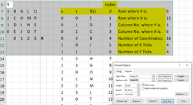
    .Offset(0, 2).Value = "x"
    .Offset(0, 3).Value = "y"
    .Offset(0, 4).Value = "f(x)"
    .Offset(0, 5).Value = 0
    .Offset(-1, 5).Value = "Index"
    Range(.Offset(0, 2), .Offset(0, 5)).Interior.Color = RGB(255, 255, 0)
    Range(.Offset(0, 2), .Offset(0, 5)).HorizontalAlignment = xlCenter
    Range(.Offset(0, 2), .Offset(0, 5)).VerticalAlignment = xlCenter

    Dim firstXCellAddress As String
    firstXCellAddress = Replace(.Offset(1, 2).Address, "$", "") 'I8

    Dim firstYCellAddress As String
    firstYCellAddress = Replace(.Offset(1, 3).Address, "$", "")  'J8

    Dim cellAddressOf0 As String
    cellAddressOf0 = Replace(.Offset(0, 5).Address, "$", "") 'L7

    Dim firstIndexCellAddress As String
    firstIndexCellAddress = Replace(.Offset(1, 5).Address, "$", "") 'L8

    Dim graphRangeAddress As String
    graphRangeAddress = graph.Address 'Graph_01

    'X formula
    .Offset(1, 2).Formula2 = "=IF(" & firstIndexCellAddress & "<>" & Chr(34) & Chr(34) & ",INT((" & firstIndexCellAddress & "-1)/(ROW(INDEX(" & graphRangeAddress & ",ROWS(" & graphRangeAddress & "),COLUMNS(" & graphRangeAddress & ")))-ROW(INDEX(" & graphRangeAddress & ",1,1))-1))," & Chr(34) & Chr(34) & ")"

    'Y formula
    .Offset(1, 3).Formula2 = "=IF(" & firstIndexCellAddress & "<>" & Chr(34) & Chr(34) & ",MOD(" & firstIndexCellAddress & "-1,ROW(INDEX(" & graphRangeAddress & ",ROWS(" & graphRangeAddress & "),COLUMNS(" & graphRangeAddress & ")))-ROW(INDEX(" & graphRangeAddress & ",1,1))-1)," & Chr(34) & Chr(34) & ")"

    'f(x) formula
    .Offset(1, 4).Formula2 = "=IF(" & firstIndexCellAddress & "<>" & Chr(34) & Chr(34) & ",INDEX(" & graphRangeAddress & ",ROW(INDEX(" & graphRangeAddress & ",ROWS(" & graphRangeAddress & "),COLUMNS(" & graphRangeAddress & ")))-ROW(INDEX(" & graphRangeAddress & ",1,1))-1-" & firstYCellAddress & "+1," & firstXCellAddress & "+2)," & Chr(34) & Chr(34) & ")"

    'Index formula
    .Offset(1, 5).Formula2 = "=IFERROR(IF(" & cellAddressOf0 & "+1<=(ROW(INDEX(" & graphRangeAddress & ",ROWS(" & graphRangeAddress & "),COLUMNS(" & graphRangeAddress & ")))-ROW(INDEX(" & graphRangeAddress & ",1,1))-1)*(COLUMN(INDEX(" & graphRangeAddress & ",ROWS(" & graphRangeAddress & "),COLUMNS(" & graphRangeAddress & ")))-COLUMN(INDEX(" & graphRangeAddress & ",1,1))-1)," & cellAddressOf0 & "+1," & Chr(34) & Chr(34) & ")," & Chr(34) & Chr(34) & ")"

    'Fill them down:
    Dim numberOfCoordinates As Long
    numberOfCoordinates = (graph(graph.Rows.Count, 1).Row - graph(1, 1).Row - 1) * (graph(graph.Rows.Count, graph.Columns.Count).column - graph(1, 1).column - 1)

    Range(.Offset(1, 2), .Offset(1 + numberOfCoordinates, 5)).Formula = Range(.Offset(1, 2), .Offset(1, 5)).Formula
   
    'Remove the formulaii
    Range(.Offset(1, 2), .Offset(1 + numberOfCoordinates, 5)).Formula = Range(.Offset(1, 2), .Offset(1 + numberOfCoordinates, 5)).Value
End With

User_Cancelled:
End Sub
Function Select_Cells(message As String)
On Error GoTo Exit_Function
Dim Selectedarea As Range
Set Selectedarea = Application.InputBox(prompt:=message & vbNewLine & vbNewLine & vbNewLine & vbNewLine, _
Title:="Select Range", Default:=Selection.Address, Type:=8)
If Not Selectedarea Is Nothing Then Set Select_Cells = Selectedarea
Exit_Function:
End Function
 
Last edited:
Upvote 0
Okay (that took longer than expected. Sorry about that.), these are the new formulas. (It turns out that you don't need to know the # of X ticks! Both x and y are dependent on the # of y ticks.)

But all I did was put the smaller formulas (in cells that no longer include formulas) into the cells that referenced them. So at least you know where these LONG formulas came from. I did modify the formula of the x's in the XY table though.

(And interestingly, if you have nothing at a specific coordinate, it will say it's 0 instead of showing a blank. So this assumes that you have every cell/coordinate filled with something.)
Blank.xlsb
IJKL
6Index
7xyf(x)0
800E1
Sheet2
Cell Formulas
RangeFormula
I8I8=IF(L8<>"",INT((L8-1)/(ROW(INDEX(Graph_01,ROWS(Graph_01),COLUMNS(Graph_01)))-ROW(INDEX(Graph_01,1,1))-1)),"")
J8J8=IF(L8<>"",MOD(L8-1,ROW(INDEX(Graph_01,ROWS(Graph_01),COLUMNS(Graph_01)))-ROW(INDEX(Graph_01,1,1))-1),"")
K8K8=IF(L8<>"",INDEX(Graph_01,ROW(INDEX(Graph_01,ROWS(Graph_01),COLUMNS(Graph_01)))-ROW(INDEX(Graph_01,1,1))-1-J8+1,I8+2),"")
L8L8=IFERROR(IF(L7+1<=(ROW(INDEX(Graph_01,ROWS(Graph_01),COLUMNS(Graph_01)))-ROW(INDEX(Graph_01,1,1))-1)*(COLUMN(INDEX(Graph_01,ROWS(Graph_01),COLUMNS(Graph_01)))-COLUMN(INDEX(Graph_01,1,1))-1),L7+1,""),"")
Named Ranges
NameRefers ToCells
Graph_01=Sheet2!$A$6:$G$11I8:L8

The formula worked like a charm, Thank you so much. :)

I added a VBA script to select the range and rename the range to Group_1

Sub generateXY()

Dim Specifiedrange As Range
Set Specifiedrange = Application.InputBox("Specifiy the range of Wafer Map", Type:=8)
MsgBox "This is the range you selected " & Specifiedrange.Address
Specifiedrange.Name = "Graph_1"

End Sub


Will try out the VBA code too. Appreciate the help. :)
 
Upvote 0
You're very welcome, but:
I added a VBA script to select the range and rename the range to Group_1

Oh, and you asked for VBA. (I somehow missed that!)

Here is the above (latest) formulaii/process translated to VBA. (No need to name a range anymore . . .
That VBA script also puts in the formulas for you. (And then converts them to values right after.)
 
Upvote 0
You're very welcome, but:


That VBA script also puts in the formulas for you. (And then converts them to values right after.)
Hi cmowla, I tried the VBA script, but there were no X/Y coordinates generated. Do I need to define any cell besides selecting the range of the graph?

1663588614315.png
 
Upvote 0
Yes, because in your original image, you had x and y labels in the graph itself, and thus that's what the script is based on. (If you change the type of input, then the program is going to naturally break.) So for it to work you would need to select all of what I see in the graph above + the first blank line above it and to the right of it.
 
Upvote 0

Forum statistics

Threads
1,214,807
Messages
6,121,679
Members
449,047
Latest member
notmrdurden

We've detected that you are using an adblocker.

We have a great community of people providing Excel help here, but the hosting costs are enormous. You can help keep this site running by allowing ads on MrExcel.com.
Allow Ads at MrExcel

Which adblocker are you using?

Disable AdBlock

Follow these easy steps to disable AdBlock

1)Click on the icon in the browser’s toolbar.
2)Click on the icon in the browser’s toolbar.
2)Click on the "Pause on this site" option.
Go back

Disable AdBlock Plus

Follow these easy steps to disable AdBlock Plus

1)Click on the icon in the browser’s toolbar.
2)Click on the toggle to disable it for "mrexcel.com".
Go back

Disable uBlock Origin

Follow these easy steps to disable uBlock Origin

1)Click on the icon in the browser’s toolbar.
2)Click on the "Power" button.
3)Click on the "Refresh" button.
Go back

Disable uBlock

Follow these easy steps to disable uBlock

1)Click on the icon in the browser’s toolbar.
2)Click on the "Power" button.
3)Click on the "Refresh" button.
Go back
Back
Top