TRANSPOSE Formula

[James8761]

Hi,

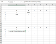
Can someone help me with a TRANSPOSE formula please. I ma trying to compare what each Division of a company reports they are owed or owe to another Division of a Company.

I've used Divisions A,B,C,D and E has an example. Division A has reported that they are owed 2,000 (A positive figure) by Division B. Division B reports that it owes Division A -100 (A negative number). A differnece of 1,900.

I am trying to put a table together underneath to show this 1,900. I have put in a formula per the image in Cell B14. Can someone tell me how to fix this please? I am using Excel O365.

Kind regards,
James

 

[EFANYoutube]

Hi James
I have used the below in the cell B14

=INDEX($A$3:$F$8,MATCH($A14,$A$3:$A$88,0),MATCH(B$12,$A$3:$F$3,0))+INDEX($A$3:$F$8,MATCH(B$12,$A$3:$A$88,0),MATCH($A14,$A$3:$F$3,0))

This is also fillable

Thanks
Excel Fan

 

[Eric W]

Try:

Book1
	A	B	C	D	E	F
1
2
3		A	B	C	D	E
4	A	-	2000
5	B	-100	-
6	C			-
7	D				-
8	E					-
9
10
11
12
13	A	2100
14	B	-2100
15	C	0
16	D	0
17	E	0
Sheet1

Cell Formulas
Range	Formula
B13:B17	B13	=SUM(INDEX($B$4:$F$8,MATCH(A13,$A$4:$A$8,0),0))-SUM(INDEX($B$4:$F$8,0,MATCH(A13,$B$3:$F$3,0)))

I came up with 2100, since if B owes 2000 to A, and B owes 100 more to A, then the total owed is 2100.

 

[James8761]

Hi James
I have used the below in the cell B14

=INDEX($A$3:$F$8,MATCH($A14,$A$3:$A$88,0),MATCH(B$12,$A$3:$F$3,0))+INDEX($A$3:$F$8,MATCH(B$12,$A$3:$A$88,0),MATCH($A14,$A$3:$F$3,0))

This is also fillable

Thanks
Excel Fan

Thanks very much, does the job.

 

[James8761]

Try:

Book1
	A	B	C	D	E	F
1
2
3		A	B	C	D	E
4	A	-	2000
5	B	-100	-
6	C			-
7	D				-
8	E					-
9
10
11
12
13	A	2100
14	B	-2100
15	C	0
16	D	0
17	E	0
Sheet1

Cell Formulas
Range	Formula
B13:B17	B13	=SUM(INDEX($B$4:$F$8,MATCH(A13,$A$4:$A$8,0),0))-SUM(INDEX($B$4:$F$8,0,MATCH(A13,$B$3:$F$3,0)))

I came up with 2100, since if B owes 2000 to A, and B owes 100 more to A, then the total owed is 2100.

Excellent, thank you very much as well.