Transpose sequence of values based on conditions

[CrisRock87]

Hello folks,

I am currently struggling to set up a macro to transpose arrays of records based on conditions.

I am quite new to VBA, so any tips and advice on how best to achieve this will be very much appreciated.

Below is the format of my 'raw' data in Excel (Version 16.0.6741.2056)

Column B contains DATETIME representing half hourly trading intervals in chronological order.
Each 'NAME' listed in column C might submit multiple offers/prices (up to 20) for each trading period.
The number of PRICE for each NAME varies each period.

A	B	C	D
1	DATETIME	NAME	PRICE
2	1/07/2015 8:00:00 AM	ALPHA	X
3	1/07/2015 8:00:00 AM	ALPHA	X
4	1/07/2015 8:00:00 AM	ALPHA	X
5	1/07/2015 8:00:00 AM	BETA	X
6	1/07/2015 8:00:00 AM	GAMMA	X
7	1/07/2015 8:00:00 AM	GAMMA	X
8	1/07/2015 8:00:00 AM	DELTA	X
9	1/07/2015 8:00:00 AM	DELTA	X
10	1/07/2015 8:00:00 AM	DELTA	X
11	1/07/2015 8:00:00 AM	DELTA	X
..	..	...
23	1/07/2015 8:30:00 AM	ALPHA	X
24	1/07/2015 8:30:00 AM	BETA	X
24	1/07/2015 8:30:00 AM	BETA	X
25	1/07/2015 8:30:00 AM	GAMMA	X
26	1/07/2015 8:30:00 AM	DELTA	X
27	1/07/2015 8:30:00 AM	DELTA	X
..	..	..	..

<tbody>
</tbody>

---

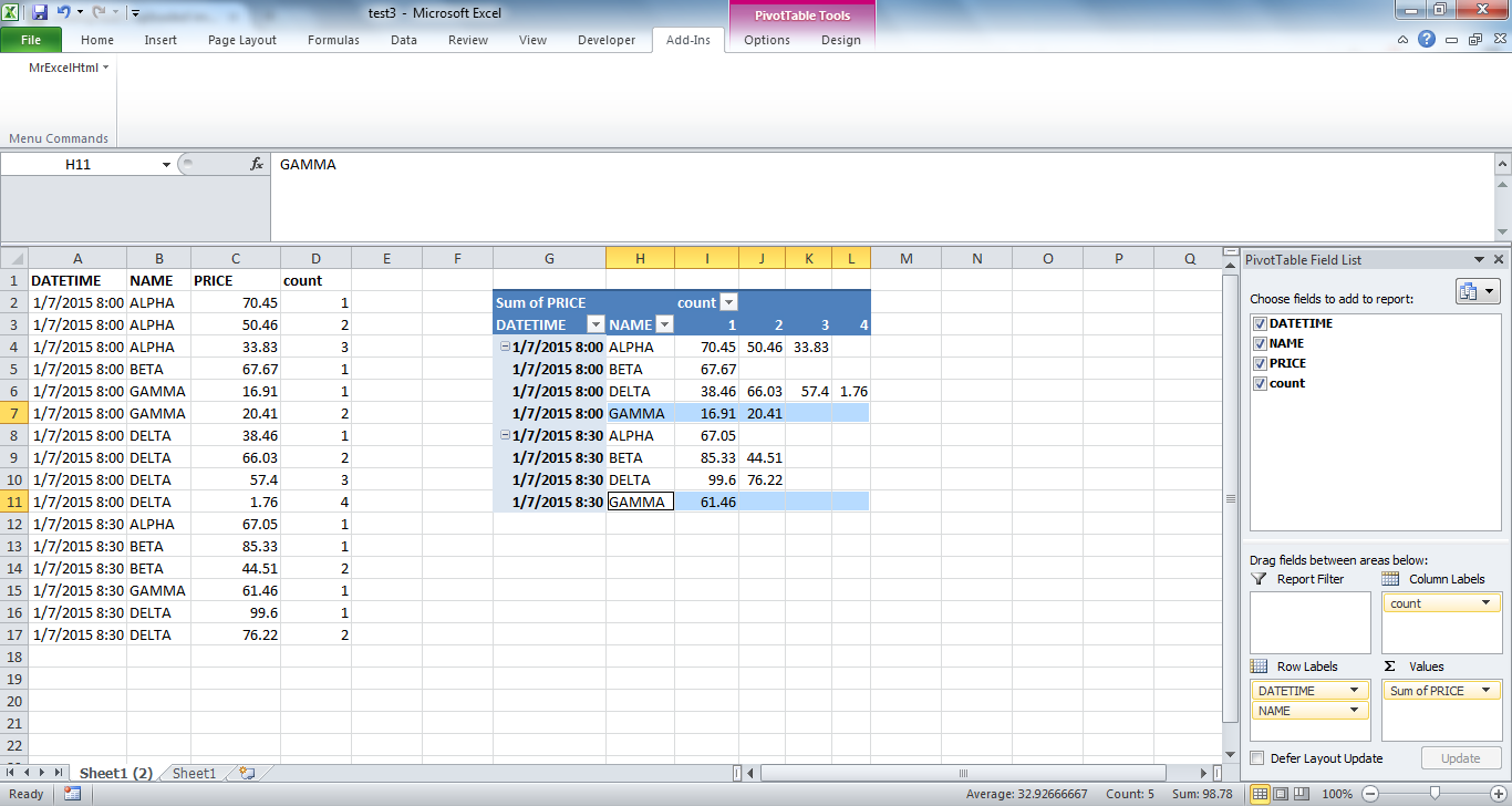
And this is what I am attempting to achieve:

For each trading period, I'd like to have for each 'NAME' the set of offers/prices reported in columns.

I've provided an example below.

A	B	C	D	E	F	G	..
1	DATETIME	NAME	PRICE 1	PRICE 2	PRICE 3	PRICE 4	..
2	1/07/2015 8:00:00 AM	ALPHA	X	X	X
3	1/07/2015 8:00:00 AM	BETA	X
4	1/07/2015 8:00:00 AM	GAMMA	X	X
5	1/07/2015 8:00:00 AM	DELTA	X	X	X	X
..	..	..
12	1/07/2015 8:30:00 AM	ALPHA	X
13	1/07/2015 8:30:00 AM	BETA	X	X
14	1/07/2015 8:30:00 AM	GAMMA	X
15	1/07/2015 8:30:00 AM	DELTA	X	X
..	..	..

<tbody>
</tbody>

---

So far I have had no luck in achieving the above.

I am dealing with a massive amount of data (several years and over hundred different "NAMES")

Any suggestion on how to streamline this process is welcome.

Thanks.

 

[sheetspread]

You don't need VBA, just remove duplicates or the advanced filter, then a formula:

Excel 2010
	A	B	C	D	E	F	G	H	I	J	K	L
1	DATETIME	NAME	PRICE
2	1/7/2015 8:00	ALPHA	70.45				1/7/2015 8:00	ALPHA	70.45	50.46	33.83
3	1/7/2015 8:00	ALPHA	50.46				1/7/2015 8:00	BETA	67.67
4	1/7/2015 8:00	ALPHA	33.83				1/7/2015 8:00	GAMMA	16.91	20.41
5	1/7/2015 8:00	BETA	67.67				1/7/2015 8:00	DELTA	38.46	66.03	57.4	1.76
6	1/7/2015 8:00	GAMMA	16.91				1/7/2015 8:30	ALPHA	67.05
7	1/7/2015 8:00	GAMMA	20.41				1/7/2015 8:30	BETA	85.33	44.51
8	1/7/2015 8:00	DELTA	38.46				1/7/2015 8:30	GAMMA	61.46
9	1/7/2015 8:00	DELTA	66.03				1/7/2015 8:30	DELTA	99.6	76.22
10	1/7/2015 8:00	DELTA	57.4
11	1/7/2015 8:00	DELTA	1.76
12	1/7/2015 8:30	ALPHA	67.05
13	1/7/2015 8:30	BETA	85.33
14	1/7/2015 8:30	BETA	44.51
15	1/7/2015 8:30	GAMMA	61.46
16	1/7/2015 8:30	DELTA	99.6
17	1/7/2015 8:30	DELTA	76.22
Sheet1

Cell Formulas
Range	Formula
I2	{=IFERROR(INDEX($C$1:$C$17,SMALL(IF($A$2:$A$17=$G2,IF($B$2:$B$17=$H2,ROW($B$2:$B$17))),COLUMN(A1))),"")}
Press CTRL+SHIFT+ENTER to enter array formulas.

 

[sheetspread]

Even better is to add a cumulative count column then set a pivot table:

Excel 2010
	A	B	C	D
1	DATETIME	NAME	PRICE	count
2	1/7/2015 8:00	ALPHA	70.45	1
3	1/7/2015 8:00	ALPHA	50.46	2
4	1/7/2015 8:00	ALPHA	33.83	3
5	1/7/2015 8:00	BETA	67.67	1
6	1/7/2015 8:00	GAMMA	16.91	1
7	1/7/2015 8:00	GAMMA	20.41	2
8	1/7/2015 8:00	DELTA	38.46	1
9	1/7/2015 8:00	DELTA	66.03	2
10	1/7/2015 8:00	DELTA	57.4	3
11	1/7/2015 8:00	DELTA	1.76	4
12	1/7/2015 8:30	ALPHA	67.05	1
13	1/7/2015 8:30	BETA	85.33	1
14	1/7/2015 8:30	BETA	44.51	2
15	1/7/2015 8:30	GAMMA	61.46	1
16	1/7/2015 8:30	DELTA	99.6	1
17	1/7/2015 8:30	DELTA	76.22	2
Sheet1 (2)

Cell Formulas
Range	Formula
D2	=COUNTIFS($A$2:A2,A2,$B$2:B2,B2)

 

[CrisRock87]

Even better is to add a cumulative count column then set a pivot table:

Excel 2010

	A	B	C	D
1	DATETIME	NAME	PRICE	count
2	1/7/2015 8:00	ALPHA	70.45	1
3	1/7/2015 8:00	ALPHA	50.46	2
4	1/7/2015 8:00	ALPHA	33.83	3
5	1/7/2015 8:00	BETA	67.67	1
6	1/7/2015 8:00	GAMMA	16.91	1
7	1/7/2015 8:00	GAMMA	20.41	2
8	1/7/2015 8:00	DELTA	38.46	1
9	1/7/2015 8:00	DELTA	66.03	2
10	1/7/2015 8:00	DELTA	57.4	3
11	1/7/2015 8:00	DELTA	1.76	4
12	1/7/2015 8:30	ALPHA	67.05	1
13	1/7/2015 8:30	BETA	85.33	1
14	1/7/2015 8:30	BETA	44.51	2
15	1/7/2015 8:30	GAMMA	61.46	1
16	1/7/2015 8:30	DELTA	99.6	1
17	1/7/2015 8:30	DELTA	76.22	2

<tbody>
</tbody>

Sheet1 (2)​

Worksheet Formulas Cell Formula D2 =COUNTIFS($A$2:A2,A2,$B$2:B2,B2) <tbody> </tbody>

<tbody>
</tbody>

Thank you very much Sheetspread,
You just saved me some trouble.
Both approaches work well and achieve exactly what I am looking for.
I was considering VBA because I am dealing with multiple csv and I have to perform this process on a regular basis.

C

 

[sheetspread]

I was considering VBA because I am dealing with multiple csv and I have to perform this process on a regular basis.

The formula/table placement can be recorded in a macro and adjusted for dynamic ranges:

Sub pricepivtab()
Dim lr%
lr = Cells(Rows.Count, 1).End(xlUp).Row
Cells(1, 4).Value = "Count"
Cells(2, 4).Resize(lr - 1).Value = "=COUNTIFS($A$2:A2,A2,$B$2:B2,B2)"

    ActiveWorkbook.PivotCaches.Create(SourceType:=xlDatabase, SourceData:= _
        Sheets("Data").Cells(1, 1).Resize(lr, 4), Version:=xlPivotTableVersion14).CreatePivotTable _
        TableDestination:=Sheets("Data").Cells(2, 6), TableName:="PivotTable2", _
        DefaultVersion:=xlPivotTableVersion14

    With ActiveSheet.PivotTables("PivotTable2")
    With .PivotFields("DATETIME")
        .Orientation = xlRowField
        .Position = 1
    End With
    With .PivotFields("NAME")
        .Orientation = xlRowField
        .Position = 2
    End With
    With .PivotFields("Count")
    .Orientation = xlColumnField
        .Position = 1
    End With
    .AddDataField .PivotFields("PRICE"), "Sum of PRICE", xlSum
        .ColumnGrand = False
        .RowGrand = False
      .RowAxisLayout xlTabularRow
      .PivotFields("DATETIME").Subtotals(1) = False
    .RepeatAllLabels xlRepeatLabels
    End With
End Sub

(I changed the sheet name to Data from Sheet1 (2) )