Treeview Parents/Child - How to return the first non blank value located one column to the left of the source cell and n rows upward.

[UlyssesFR]

Hi all, I'll try to be as clear as possible so please do not hesitate to ask for clarification.

I'm working with a text file data extracted from CATIA V5 that replicates the tree structure of an assembly with its components and subcomponents.

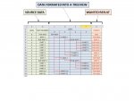
From that text file I arranged the source data in column A and B in such a way:

• Column A contains the assembly level (0 being the top assembly all the way down to level 3)
• Column B contains the component's part number or name

I have formatted that data in a more visual way in columns C to F to replicate a treeview structure:

• So column C has the top assembly at level 0
• Column D has all the sub-components at level 1
• Column E, level 2 sub-components
• Column F, level 3 sub-components

This formatting was achieved by using the following formula:

• Cell C3 for example is =IF($C$2=VALUE(A3),B3,"DELETE")
• This formula was then pasted across columns C to F cells.
• I then run a VBA macro that clears the content of all cells containing the DELETE value to make sure all unused cells in columns C to F are truly empty.

Now... What I'm trying to achieve is to return the parent component of each component in their corresponding row (eee the attached picture to see the wanted results)

For example for SUB-ASSY 1 row 5; I would like cell G5 to return the value ASSY 1 (contained in cells B4 or D4)
Another example in PART 10 row 17; I would like cell G17 to return the value TOP ASSY (contained in cells B3 or C3)

I'm not sure if that could be achieved by just using the source data column A and B:

I'm thinking for example, cell G12 looks at the value of cell A12 (in that case 1) then looks upward for the first value that is equal to the value in cell A12 minus 1 (in that case 0) which would be in cell A3 and then returns the value in the cell adjacent to it (in that case cell B3 = TOP ASSY)

Or if this could be achieved using the formatted data in column C to F:

I'm thinking for example, cell G12 looks in range C12:F12 for a non-empty cell (in that case cell D12), then goes one column to the left (Column C) and n rows upward until it meets the first non-empty cell (in that case cell C3) and returns its value (TOP ASSY)

Unfortunately, I've been looking at this for a while now and I'm no closer to finding a solution

I hope you can help me, thank you for your time

Kind regards,

 

[braindiesel]

Something like this...

Book4
	D	E	F	G	H	I
1		DATA TYPE	0	1	2	3
2	0	Data1	Data1
3	1	Data2		Data2
4	2	Data3			Data3
5	3	Data4				Data4
6	0	Data5	Data5
7	0	Data6	Data6
8	0	Data7	Data7
9	3	Data8				Data8
10	3	Data9				Data9
11	2	Data10			Data10
Sheet2

Cell Formulas
Range	Formula
F2:I11	F2	=IF($D2=F$1,$E2,"")

 

[UlyssesFR]

Something like this...

Book4
	D	E	F	G	H	I
1		DATA TYPE	0	1	2	3
2	0	Data1	Data1
3	1	Data2		Data2
4	2	Data3			Data3
5	3	Data4				Data4
6	0	Data5	Data5
7	0	Data6	Data6
8	0	Data7	Data7
9	3	Data8				Data8
10	3	Data9				Data9
11	2	Data10			Data10
Sheet2

Cell Formulas
Range	Formula
F2:I11	F2	=IF($D2=F$1,$E2,"")

Ok it seems I have overcomplicated my question by detailing how I got there.

I already have the data you are showing in your table.

Maybe it'll make more sense if I use the Directory/Sub-Directory analogy.

What formula in column G would allow me to display the parent directory as shown in the table below?

TREEVIEW.xlsx
	A	B	C	D	E	F	G
1	LEVEL	DIRECTORY	LEVEL				PARENT DIRECTORY
2			0	1	2	3
3	0	ROOT DIRECTORY	ROOT DIRECTORY
4	1	SUB-DIRECTORY A		SUB-DIRECTORY A			ROOT DIRECTORY
5	2	SUB-DIRECTORY AA			SUB-DIRECTORY AA		SUB-DIRECTORY A
6	3	SUB-DIRECTORY AA1				SUB-DIRECTORY AA1	SUB-DIRECTORY AA
7	3	SUB-DIRECTORY AA2				SUB-DIRECTORY AA2	SUB-DIRECTORY AA
8	3	SUB-DIRECTORY AA3				SUB-DIRECTORY AA3	SUB-DIRECTORY AA
9	3	SUB-DIRECTORY AA4				SUB-DIRECTORY AA4	SUB-DIRECTORY AA
10	2	SUB-DIRECTORY AB			SUB-DIRECTORY AB		SUB-DIRECTORY A
11	2	SUB-DIRECTORY AC			SUB-DIRECTORY AC		SUB-DIRECTORY A
12	1	SUB-DIRECTORY B		SUB-DIRECTORY B			ROOT DIRECTORY
13	2	SUB-DIRECTORY BA			SUB-DIRECTORY BA		SUB-DIRECTORY B
14	3	SUB-DIRECTORY BA1				SUB-DIRECTORY BA1	SUB-DIRECTORY BA
15	3	SUB-DIRECTORY BA2				SUB-DIRECTORY BA2	SUB-DIRECTORY BA
16	3	SUB-DIRECTORY BA3				SUB-DIRECTORY BA3	SUB-DIRECTORY BA
17	1	SUB-DIRECTORY C		SUB-DIRECTORY C			ROOT DIRECTORY
18	1	SUB-DIRECTORY D		SUB-DIRECTORY D			ROOT DIRECTORY
Book1 (2)

Cell Formulas
Range	Formula
C3:F18	C3	=IF(C$2=$A3,$B3,"")

 

[Peter_SSs]

Welcome to the MrExcel board!

Try this, copied down.

20 07 01.xlsm
	A	B	C	D	E	F	G
1	LEVEL	DIRECTORY	LEVEL				PARENT DIRECTORY
2			0	1	2	3
3	0	ROOT DIRECTORY	ROOT DIRECTORY
4	1	SUB-DIRECTORY A		SUB-DIRECTORY A			ROOT DIRECTORY
5	2	SUB-DIRECTORY AA			SUB-DIRECTORY AA		SUB-DIRECTORY A
6	3	SUB-DIRECTORY AA1				SUB-DIRECTORY AA1	SUB-DIRECTORY AA
7	3	SUB-DIRECTORY AA2				SUB-DIRECTORY AA2	SUB-DIRECTORY AA
8	3	SUB-DIRECTORY AA3				SUB-DIRECTORY AA3	SUB-DIRECTORY AA
9	3	SUB-DIRECTORY AA4				SUB-DIRECTORY AA4	SUB-DIRECTORY AA
10	2	SUB-DIRECTORY AB			SUB-DIRECTORY AB		SUB-DIRECTORY A
11	2	SUB-DIRECTORY AC			SUB-DIRECTORY AC		SUB-DIRECTORY A
12	1	SUB-DIRECTORY B		SUB-DIRECTORY B			ROOT DIRECTORY
13	2	SUB-DIRECTORY BA			SUB-DIRECTORY BA		SUB-DIRECTORY B
14	3	SUB-DIRECTORY BA1				SUB-DIRECTORY BA1	SUB-DIRECTORY BA
15	3	SUB-DIRECTORY BA2				SUB-DIRECTORY BA2	SUB-DIRECTORY BA
16	3	SUB-DIRECTORY BA3				SUB-DIRECTORY BA3	SUB-DIRECTORY BA
17	1	SUB-DIRECTORY C		SUB-DIRECTORY C			ROOT DIRECTORY
18	1	SUB-DIRECTORY D		SUB-DIRECTORY D			ROOT DIRECTORY
Parent

Cell Formulas
Range	Formula
G3:G18	G3	=IF(A3=0,"",INDEX(B$2:B2,AGGREGATE(14,6,(ROW(B$2:B2)-ROW(B$2)+1)/(A$2:A2=A3-1),1)))

 

[UlyssesFR]

Welcome to the MrExcel board!

Try this, copied down.

20 07 01.xlsm
	A	B	C	D	E	F	G
1	LEVEL	DIRECTORY	LEVEL				PARENT DIRECTORY
2			0	1	2	3
3	0	ROOT DIRECTORY	ROOT DIRECTORY
4	1	SUB-DIRECTORY A		SUB-DIRECTORY A			ROOT DIRECTORY
5	2	SUB-DIRECTORY AA			SUB-DIRECTORY AA		SUB-DIRECTORY A
6	3	SUB-DIRECTORY AA1				SUB-DIRECTORY AA1	SUB-DIRECTORY AA
7	3	SUB-DIRECTORY AA2				SUB-DIRECTORY AA2	SUB-DIRECTORY AA
8	3	SUB-DIRECTORY AA3				SUB-DIRECTORY AA3	SUB-DIRECTORY AA
9	3	SUB-DIRECTORY AA4				SUB-DIRECTORY AA4	SUB-DIRECTORY AA
10	2	SUB-DIRECTORY AB			SUB-DIRECTORY AB		SUB-DIRECTORY A
11	2	SUB-DIRECTORY AC			SUB-DIRECTORY AC		SUB-DIRECTORY A
12	1	SUB-DIRECTORY B		SUB-DIRECTORY B			ROOT DIRECTORY
13	2	SUB-DIRECTORY BA			SUB-DIRECTORY BA		SUB-DIRECTORY B
14	3	SUB-DIRECTORY BA1				SUB-DIRECTORY BA1	SUB-DIRECTORY BA
15	3	SUB-DIRECTORY BA2				SUB-DIRECTORY BA2	SUB-DIRECTORY BA
16	3	SUB-DIRECTORY BA3				SUB-DIRECTORY BA3	SUB-DIRECTORY BA
17	1	SUB-DIRECTORY C		SUB-DIRECTORY C			ROOT DIRECTORY
18	1	SUB-DIRECTORY D		SUB-DIRECTORY D			ROOT DIRECTORY
Parent

Cell Formulas
Range	Formula
G3:G18	G3	=IF(A3=0,"",INDEX(B$2:B2,AGGREGATE(14,6,(ROW(B$2:B2)-ROW(B$2)+1)/(A$2:A2=A3-1),1)))

This is amazing and is exactly what I am looking for.

Unfortunately, in my attempt to simplify my request I seem to halve altered/omitted the nature/source of some of the cells/ranges you are using in the formula.

As a result, I am getting a #NUM error upon pasting the formula.

Please find the actual worksheet I'm working from below:

N254L4001-000_CATIA V5_TREE FORMATING FROM LISTING REPORT_20200701_0940.xlsm
	A	B	C	D	E	F	G	H	I	J	K	L	M	N
2	RAW	TRIMMED	LVL	PART NUMBER	0	1	2	3	4	5	6	7	8	USED IN
3	0 N254L4001-000	0 N254L4001-000	0	N254L4001-000	N254L4001-000									#NUM!
4	1 N254L4002-000	1 N254L4002-000	1	N254L4002-000		N254L4002-000								#NUM!
5	2 N254L4003-000	2 N254L4003-000	2	N254L4003-000			N254L4003-000							#NUM!
6	3 N254L4055-000	3 N254L4055-000	3	N254L4055-000				N254L4055-000						#NUM!
7	4 N254L5002-200	4 N254L5002-200	4	N254L5002-200					N254L5002-200					#NUM!
8	4 N254L5029-200	4 N254L5029-200	4	N254L5029-200					N254L5029-200					#NUM!
9	3 N254L4057-000	3 N254L4057-000	3	N254L4057-000				N254L4057-000						#NUM!
10	4 N254L5003-200	4 N254L5003-200	4	N254L5003-200					N254L5003-200					#NUM!
11	4 N254L5030-200	4 N254L5030-200	4	N254L5030-200					N254L5030-200					#NUM!
12	4 N254L5036-200	4 N254L5036-200	4	N254L5036-200					N254L5036-200					#NUM!
13	4 N254L5036-200	4 N254L5036-200	4	N254L5036-200					N254L5036-200					#NUM!
14	4 N254L5036-200	4 N254L5036-200	4	N254L5036-200					N254L5036-200					#NUM!
15	3 N254L4058-000	3 N254L4058-000	3	N254L4058-000				N254L4058-000						#NUM!
16	4 N254L5005-200	4 N254L5005-200	4	N254L5005-200					N254L5005-200					#NUM!
17	4 N254L5036-200	4 N254L5036-200	4	N254L5036-200					N254L5036-200					#NUM!
18	4 N254L5036-200	4 N254L5036-200	4	N254L5036-200					N254L5036-200					#NUM!
19	4 N254L5036-200	4 N254L5036-200	4	N254L5036-200					N254L5036-200					#NUM!
20	4 N254L5036-200	4 N254L5036-200	4	N254L5036-200					N254L5036-200					#NUM!
21	4 N254L5103-200	4 N254L5103-200	4	N254L5103-200					N254L5103-200					#NUM!
22	4 N254L5296-200	4 N254L5296-200	4	N254L5296-200					N254L5296-200					#NUM!
23	4 N254L5299-200	4 N254L5299-200	4	N254L5299-200					N254L5299-200					#NUM!
24	3 N254L4059-000	3 N254L4059-000	3	N254L4059-000				N254L4059-000						#NUM!
FORMATED

Cell Formulas
Range	Formula
B3:B24	B3	=TRIM(A3)
C3:C24	C3	=LEFT(B3,1)
D3:D24	D3	=RIGHT(B3,LEN(B3)-2)
E3	E3	=IF($E$2=VALUE(C3),D3,"DELETE")
F4	F4	=IF($F$2=VALUE(C4),D4,"DELETE")
G5	G5	=IF($G$2=VALUE(C5),D5,"DELETE")
H6,H24,H15,H9	H6	=IF($H$2=VALUE(C6),D6,"DELETE")
I16:I23,I10:I14,I7:I8	I7	=IF($I$2=VALUE(C7),D7,"DELETE")
N3:N24	N3	=IF(C3=0,"",INDEX(D$2:D2,AGGREGATE(14,6,(ROW(D$2:D2)-ROW(D$2)+1)/(C$2:C2=C3-1),1)))

 

[Peter_SSs]

Your values in column C are text, not numerical, as formula was expecting.
Can you alter your C3 formula to this & copy down?
=LEFT(B3,1)+0

Then your existing formulas in column N should return the correct results I think.

Further, if you make that change, then you shouldn't need the VALUE() function in your columns E:I formulas.
In E3, it would only need ..
=IF($E$2=C3,D3,"DELETE")
.. which is more like what you had in post #3.

BTW, why are you using "DELETE" in that formula and not just
=IF($E$2=C3,D3,"")

 

[UlyssesFR]

Your values in column C are text, not numerical, as formula was expecting.
Can you alter your C3 formula to this & copy down?
=LEFT(B3,1)+0

Then your existing formulas in column N should return the correct results I think.

Indeed you are right, flawless, perfect! Thank you so much!!!

Now I'm going to stare at this function for weeks and try to dissect it in order to understand how it works, but INDEX and AGGREGATE are so obscure to me.

 

[Peter_SSs]

You're welcome.

Did you see the edits I added that perhaps happened after you initially viewed my previous post?

 

[UlyssesFR]

You're welcome.

Did you see the edits I added that perhaps happened after you initially viewed my previous post?

I had not seen the edits.

I'm using DELETE in the formula =IF($E$2=C3,D3,"DELETE") because I needed the cell to be truly empty instead of containing a ""

So I have a bit of VBE that clears the content of all cells within my range afterward.

' Clear Content of Cells containing DELETE in the Tree View Range'
    For Each cell In ActiveSheet.Range("A1", ActiveCell.SpecialCells(xlLastCell))
        If cell.Value = "DELETE" Then
           cell.ClearContents
        End If
    Next cell

This allows my tree to look like this (the text carries into the next column because the adjacent cell is now truly empty):

Instead of like this (the text stops as far as the width of the column goes, because the next cell contains "" and thus is not truly empty):

As for removing the VALUE(), thanks, I have removed it and nothing collapsed

Thanks again!

 

[UlyssesFR]

VBA, not VBE...

Not sure how to edit a post once it's been posted...