Hi all, I'll try to be as clear as possible so please do not hesitate to ask for clarification.
I'm working with a text file data extracted from CATIA V5 that replicates the tree structure of an assembly with its components and subcomponents.
From that text file I arranged the source data in column A and B in such a way:
I have formatted that data in a more visual way in columns C to F to replicate a treeview structure:
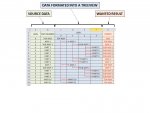
Now... What I'm trying to achieve is to return the parent component of each component in their corresponding row (eee the attached picture to see the wanted results)
For example for SUB-ASSY 1 row 5; I would like cell G5 to return the value ASSY 1 (contained in cells B4 or D4)
Another example in PART 10 row 17; I would like cell G17 to return the value TOP ASSY (contained in cells B3 or C3)
I'm not sure if that could be achieved by just using the source data column A and B:
I'm thinking for example, cell G12 looks at the value of cell A12 (in that case 1) then looks upward for the first value that is equal to the value in cell A12 minus 1 (in that case 0) which would be in cell A3 and then returns the value in the cell adjacent to it (in that case cell B3 = TOP ASSY)
Or if this could be achieved using the formatted data in column C to F:
I'm thinking for example, cell G12 looks in range C12:F12 for a non-empty cell (in that case cell D12), then goes one column to the left (Column C) and n rows upward until it meets the first non-empty cell (in that case cell C3) and returns its value (TOP ASSY)
Unfortunately, I've been looking at this for a while now and I'm no closer to finding a solution
I hope you can help me, thank you for your time
Kind regards,
I'm working with a text file data extracted from CATIA V5 that replicates the tree structure of an assembly with its components and subcomponents.
From that text file I arranged the source data in column A and B in such a way:
- Column A contains the assembly level (0 being the top assembly all the way down to level 3)
- Column B contains the component's part number or name
I have formatted that data in a more visual way in columns C to F to replicate a treeview structure:
- So column C has the top assembly at level 0
- Column D has all the sub-components at level 1
- Column E, level 2 sub-components
- Column F, level 3 sub-components
- Cell C3 for example is =IF($C$2=VALUE(A3),B3,"DELETE")
- This formula was then pasted across columns C to F cells.
- I then run a VBA macro that clears the content of all cells containing the DELETE value to make sure all unused cells in columns C to F are truly empty.
Now... What I'm trying to achieve is to return the parent component of each component in their corresponding row (eee the attached picture to see the wanted results)
For example for SUB-ASSY 1 row 5; I would like cell G5 to return the value ASSY 1 (contained in cells B4 or D4)
Another example in PART 10 row 17; I would like cell G17 to return the value TOP ASSY (contained in cells B3 or C3)
I'm not sure if that could be achieved by just using the source data column A and B:
I'm thinking for example, cell G12 looks at the value of cell A12 (in that case 1) then looks upward for the first value that is equal to the value in cell A12 minus 1 (in that case 0) which would be in cell A3 and then returns the value in the cell adjacent to it (in that case cell B3 = TOP ASSY)
Or if this could be achieved using the formatted data in column C to F:
I'm thinking for example, cell G12 looks in range C12:F12 for a non-empty cell (in that case cell D12), then goes one column to the left (Column C) and n rows upward until it meets the first non-empty cell (in that case cell C3) and returns its value (TOP ASSY)
Unfortunately, I've been looking at this for a while now and I'm no closer to finding a solution
I hope you can help me, thank you for your time
Kind regards,


