Trouble making chart dynamic

[riedyp]

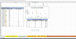
Trying to make my "time spent versus time allocated chart" update when new values are inputted in the chart below it.
Cells K35:N60 are populated with formulas that will only show a value if they are inputted on another sheet.

K35: =IF(ROW()-ROW(K$34)<=SUM(IFERROR(--(('Project - Gantt Chart'!$B$9:$B$45/INT('Project - Gantt Chart'!$B$9:$B$45))=1),"")),ROW()-ROW(K$34),"")
L35: =IFERROR(INDEX('Project - Gantt Chart'!$B$9:$I$45,MATCH('Executive Summary'!$K35,'Project - Gantt Chart'!$B$9:$B$45,0),4),"")
M35: =IFERROR(INDEX('Project - Gantt Chart'!$B$9:$I$45,MATCH('Executive Summary'!$K35,'Project - Gantt Chart'!$B$9:$B$45,0),5),"")
N35: =IFERROR(INDEX('Project - Gantt Chart'!$B$9:$I$45,MATCH('Executive Summary'!$K35,'Project - Gantt Chart'!$B$9:$B$45,0),8),"")

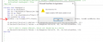
Below is the code I have been trying to use. I don't really have any other insights on how to go about this so any suggestion would be more than welcomed! Thank you.

Private Sub TimeSpent()
Dim ch As ChartObject
Set ch = Worksheets("Executive Summary").ChartObjects("Chart 8")
LastRow = Worksheets("Executive Summary").Columns("J").Find(1, SearchDirection:=xlPrevious, LookIn:=xlValues, LookAt:=xlWhole).Row

Worksheets("Executive Summary").ChartObjects("Chart 8").Activate

    ActiveChart.SeriesCollection.NewSeries
    ActiveChart.FullSeriesCollection(1).Name = Worksheets("Executive Summary").Range("L34")
    ActiveChart.FullSeriesCollection(1).Values = Range(Cells(35, 12), Cells(LastRow, 12))
    ActiveChart.SeriesCollection.NewSeries
    ActiveChart.FullSeriesCollection(2).Name = Worksheets("Executive Summary").Range("M34")
    ActiveChart.FullSeriesCollection(2).Values = Range(Cells(35, 13), Cells(LastRow, 13))
    ActiveChart.HasLegend = True
End Sub

 

[Jon Peltier]

What are the series in the chart?
Do the series names change, or just the number of points in each series?

It looks like you want two series:
=SERIES('Executive Summary'!$L$34,'Executive Summary'!$K$35:$K$40,'Executive Summary'!$L$35:$L$40,1)
=SERIES('Executive Summary'!$M$34,'Executive Summary'!$K$35:$K$40,'Executive Summary'!$M$35:$M$40,2)

When phase 7 is added, the last row will become 41. Assuming your code discovers it correctly (if column J includes formulas that look like "" when there's nothing in the other worksheet, it might not), then your code could be as simple as this:

Private Sub TimeSpent()
    Dim ws As Worksheet
    Set ws = Worksheets("Executive Summary")
    Dim ch As Chart
    Set ch = ws.ChartObjects("Chart 8").Chart
    Dim LastRow As Long
    LastRow = ws.Columns("J").Find("*", SearchDirection:=xlPrevious, LookIn:=xlValues, LookAt:=xlWhole).Row

    ch.SeriesCollection(1).XValues = ws.Range(ws.Cells(35, 11), ws.Cells(LastRow, 11))
    ch.SeriesCollection(1).Values = ws.Range(ws.Cells(35, 12), ws.Cells(LastRow, 12))

    ' don't need to repeat XValues, which are shared by all series
    ch.SeriesCollection(2).Values = ws.Range(ws.Cells(35, 13), ws.Cells(LastRow, 13))
End Sub

 

[riedyp]

Hello,

any idea why i keep getting this error? Your code looks like it is exactly what i want to accomplish.

 

[Jon Peltier]

Oops, didn't test it, just copied what you started with.

I changed

.Find(1,

to

.Find("*",

and the error went away.

 

[riedyp]

Hm, I still encounter the same error message for some reason, any idea why this may be occuring?

This is the what the formula is in cells in column J. So J35=IF(K35<>"",1,"")

 

[riedyp]

Would it be because I did not "Set" "LastRow" ? Because when i do "Set" it i get the error "Object required".

 

[Jon Peltier]

No, it's not "Set".

These two lines work fine for me, with the same kind of formula in column J:

    Dim LastRow As Long
    LastRow = ws.Columns("J").Find("*", SearchDirection:=xlPrevious, LookIn:=xlValues, LookAt:=xlWhole).Row

 

[riedyp]

Thank you, it worked. The reason I was having issues is because I changed the formatting of the all of the "1"s in column J to be hidden with ";;;" but that caused the error. So I just switched their text color to white and it worked fine. Is there a way for me to make this code be autoupdated when any changes are made?

 

[Jon Peltier]

Right click on this worksheet's tab, and select View Code. When the code module for the worksheet appears, select Worksheet from the left-hand dropdown at the top of the window, then select Calculate from the right-hand dropdown. In the Worksheet_Calculate stub that is generated, enter the name of this procedure. Whenever a value on this worksheet changes because of a calculation, the Worksheet_Calculate sub will run, and this will run your other code.

 

[Jon Peltier]

Here's another approach that doesn't require VBA, and it updates automatically when the data updates. It uses Names (a/k/a "named ranges") that grow with the data.

I've added a formula in cell J34:
=COUNT(J35:J65)
which counts the number of cells in column J next to the data that contain a numeric value. This formula doesn't care if you use a number format of ;;; to prevent the numbers from displaying, it counts the underlying values. This cell tells me how many rows are in the Names.

Go to the Formulas tab, click Define Name. In the dialog enter these:

Name: Phase
Refers To:
=OFFSET($K$34,1,0,$J$34,1)

This means Phase is the name of the range that, with respect to $K$34 starts one row down and zero columns right, and it is $J$34 rows high and 1 column wide. So in your screenshot, it is range K35:K40.

Add these two Names:

Name: HoursAllocated
Refers To:
=OFFSET(Phase,0,1)

Name: HoursSpent
Refers To:
=OFFSET(Phase,0,2)

So HoursAllocated is the range zero rows down and one column to the right of Phase (if you don't specify height and width, it uses the size of the reference range Phase), and HoursSpent is the range zero rows down and two columns to the right.

Make your chart. It should have two series with these series formulas:
=SERIES('Executive Summary'!$L$34,'Executive Summary'!$K$35:$K$40,'Executive Summary'!$L$35:$L$40,1)
=SERIES('Executive Summary'!$M$34,'Executive Summary'!$K$35:$K$40,'Executive Summary'!$M$35:$M$40,2)

Edit these right in the formula bar so you have:
=SERIES('Executive Summary'!$L$34,'Executive Summary'!Phase,'Executive Summary'!HoursAllocated,1)
=SERIES('Executive Summary'!$M$34,'Executive Summary'!Phase,'Executive Summary'!HoursSpent,2)

After you hit Enter for each formula, Excel changes 'Executive Summary' in front of each Name to the workbook name, but that's not an issue. Also, you don't need to change K35:K40 to Phase in the second formula, since Excel uses the same X values for both series in a column chart.

When the data updates and another 1 is added to column J, cell J34 increases by one, the Names extend one row lower, and the chart updates accordingly.