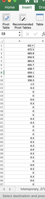
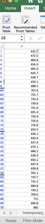
So I have a very long column of data - several thousand rows most of which = close to 0. Between every 140 and 170 (not the same gap every time!) rows I have between 9 and 11 data points that I need. If I use a data filter I get the information I need but i have no way to convert that into multiple columns containing those points. I hope that makes sense, please let me know if you have any ideas!
-
If you would like to post, please check out the MrExcel Message Board FAQ and register here. If you forgot your password, you can reset your password.
Turning filtered data into columns
- Thread starter henrycm
- Start date
Similar threads
- Solved
- Question


