Hi everyone, I'm dealing with an issue cause I can't set an array formula to a range.
This is my formula
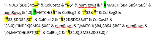
As my ranges are dynamics I managed this way on VBA
But when I get this point, the message of the title appears.
Also I tried parting the formula into two and making a replace like below but didn't work.
Please help me, I'm dealing with this issue for months.
This is my formula
VBA Code:
=INDEX($AA$4:$EC$1389, MATCH($B4,$B$4:$B$1389,0), MATCH($EN$2&EN$3,$AA$2:$EC$2&$AA$3:$EC$3,0))*INDEX($M$4:$X$1389,MATCH($B4,$B$4:$B$1389,0),MATCH(LEFT($EN$2,3),$M$3:$X$3,0))As my ranges are dynamics I managed this way on VBA
VBA Code:
Cells(4, ColCost + 9).FormulaArray = "=INDEX($DD$4:$ " & ColCost2 & " $" & numRows & ", MATCH($B4,$B$4:$B$" & numRows & ",0), MATCH($ " & ColBeg2 & " $2& " & ColBeg2 & " $3,$DD$2:$ " & ColCost2 & " $2&$DD$3:$" & ColCost2 & "$3,0))*INDEX($M$4:$X$" & numRows & ",MATCH($B4,$B$4:$B$" & numRows & ",0),MATCH(LEFT($ " & ColBeg2 & " $2,3),$M$3:$X$3,0))"But when I get this point, the message of the title appears.
Also I tried parting the formula into two and making a replace like below but didn't work.
VBA Code:
Dim theFormulaPart1 As String
     Dim theFormulaPart2 As String
     theFormulaPart1 = "=INDEX($DD$4:$ " & ColCost2 & " $" & numRows & ", MATCH($B4,$B$4:$B$" & numRows & ",0),""X_X_X)"")"

     theFormulaPart2 = "MATCH($ " & ColBeg2 & " $2& " & ColBeg2 & " $3,$DD$2:$ " & ColCost2 & " $2&$DD$3:$" & ColCost2 & "$3,0))*INDEX($M$4:$X$" & numRows & ",MATCH($B4,$B$4:$B$" & numRows & ",0),MATCH(LEFT($ " & ColBeg2 & " $2,3),$M$3:$X$3,0))"
     With Cells(4, ColCost + 9)
         .FormulaArray = theFormulaPart1
        .Replace """X_X_X)"")", theFormulaPart2
Please help me, I'm dealing with this issue for months.
")