Unconventional Index-Match-Match question

[scoveg13]

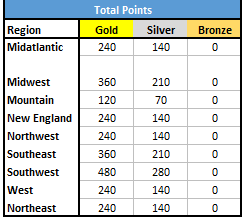
Please use the chart below as reference.

I'm trying to do an If- Index-Match-Match formula based on the chart below. Instead of pulling the numbers, I need to Index the "Gold, Silver, Bronze" column. Example, if Midatlantic has 60 points, then Silver will be the returned result.

=INDEX(U3:W3,MATCH(A20,T4:T12,1),MATCH(E20,U4:W12,1))

where U3:W3 = Gold, Silver Bronze,
a20, t4-t12= Region
e20,U4:W12 = Points.


Region Gold Silver Bronze
Midatlantic 100 60 40
Midwest 150 90 60
Mountain 50 30 20
New England 100 60 40
Northwest 100 60 40
Southeast 150 90 60
Southwest 200 120 80
West 100 60 40
Northeast 100 60 40

Any help would be greatly appreciated.

 

[AhoyNC]

Try:

Excel Workbook
	A	E	T	U	V	W
2
3			Region	Gold	Silver	Bronze
4			Midatlantic	100	60	40
5			Midwest	150	90	60
6			Mountain	50	30	20
7			New England	100	60	40
8			Northwest	100	60	40
9			Southeast	150	90	60
10			Southwest	200	120	80
11			West	100	60	40
12			Northeast	100	60	40
18
19			Silver
20	Midatlantic	60
Sheet

 

[Taul]

Hi AhoyNC,
I was getting a slight glitch on the use of the formula.
The only way I could get it work with numbers in-between the grid values was to change one of the match types from 0 to 1
and to reverse the table headers from "Gold, Silver, Bronze" to "Bronze, Silver, Gold"

=INDEX($U$3:$W$3,MATCH($E$20,INDEX($U$4:$W$12,MATCH($A$20,$T$4:$T$12,0),0),1))

Paul.

 

[AhoyNC]

@Taul,
I think if you change the 1 to a -1 in your formula you will not have to reverse the table headers, but would depend on range for Gold, Silver & Bronze.

Excel Workbook
	A	E	F	S	T	U	V	W
3					Region	Gold	Silver	Bronze
4					Midatlantic	100	60	40
5					Midwest	150	90	60
6					Mountain	50	30	20
7					New England	100	60	40
8					Northwest	100	60	40
9					Southeast	150	90	60
10					Southwest	200	120	80
11					West	100	60	40
12					Northeast	100	60	40
13
14
15
16
17
18
19				Silver
20	Midatlantic	55
Sheet

 

[Taul]

Hi AhoyNC,
For Midatlantic, if you score 55 it should return Bronze (as you need 60 or more to get to silver)

Paul

 

[Aladin Akyurek]

Hi AhoyNC,
For Midatlantic, if you score 55 it should return Bronze (as you need 60 or more to get to silver)

Paul

Looks like you are thinking along the following lines...

Row\Col	A​	E​	F​	T​	U​	V​	W​
3​				Region	Bronze	Silver	Gold
4​				Midatlantic	40​	60​	100​
5​				Midwest	60​	90​	150​
6​				Mountain	20​	30​	50​
7​				New England	40​	60​	100​
8​				Northwest	40​	60​	100​
9​				Southeast	60​	90​	150​
10​				Southwest	80​	120​	200​
11​				West	40​	60​	100​
12​				Northeast	40​	60​	100​
13​
20​	Midatlantic	60​	Silver
21​	Midatlantic	55​	Bronze
22​	Midatlantic	100​	Gold
23​	Midatlantic	40​	Bronze
24​	Midatlantic	30​	#N/A​
25​	Midatlantic	75​	Silver

Note the reorganization of the table in ascending order!...

In F20 enter and copy down:

=INDEX($U$3:$W$3,MATCH(E20,INDEX($U$4:$W$12,MATCH(A20,$T$4:$T$12,0),0),1)-
    (LOOKUP(E20,INDEX($U$4:$W$12,MATCH(A20,$T$4:$T$12,0),0))>E20))

 

[scoveg13]

Wow thank you everyone! This worked beautifully.

Now there's a Part 2 to this question. I'm using TWO tables, not just one. The table above is the "New Points" criteria. I have a second table that has the same format, regions, points, gold silver bronze, etc, but the points are higher as these are considered "Total" points (add 100 to the New Points to use a theoretical "Total Points" as the values don't matter.

Here's the logic:

If New Points is silver and Total Points is Gold - Default to Silver. If New Points is Gold and Total points is Silver, default to silver. The lower of the "metals" is picked based on the point values. So essentially, it looks like I'd have to use the same index, match, lookup formula again on the "Total Points" table, the issue is integrating the two index-match-lookup formulas WITH the given logic at the start of this paragraph. I hope this makes sense. In my world, I have "New points" at e20, "Total Points" as f20 and The "gold, silver, bronze" - index-match-lookup formula at g20.

 

[Aladin Akyurek]

What did you opt for?

Involving your second question, would you post a table of correspondences you seem to describe?

 

[scoveg13]

What did you opt for?

Involving your second question, would you post a table of correspondences you seem to describe?

I opted for this formula: =INDEX(U3:W3,MATCH(E20,INDEX(U4:W12,MATCH(A20,T4:T12,0),0),1)-(LOOKUP(E20,INDEX(U4:W12,MATCH(A20,T4:T12,0),0))>E20))

 

[Aladin Akyurek]

Ok. Would you repost the table such that it is not needed to retype it. Is this the second table you talk about?