Unique Value in a Range

[Denny57]

I am trying to identify the cell in a row which contains a unique but specific value or if that value is not unique then to return a zero value

Example 1 Find Value "C" (unique in range)

Range: A1:A5
Cell Values: A1=B, A2 =C, A3 =D, A4 =E & A5 =F
Find the unique cell that contains Value "C" and indicate in Cell B1 (Show cell reference eg. A2)

Example 2 Find Value "C" (Not unique in range)

Range: A1:A5
Cell Values: A1=B, A2 =C, A3 =C, A4 =E & A5 =F
Identifies that value "C" is not unique and returns "0" in Cell B1 (Show 0), if not 0 then a suitable "Not Found" indicator

If a unique specified value is identifed then I will need to use the cell refernce containing this unique value in a subsequent calculation.

Any help is greatly appreciated

 

[Phuoc]

Try this:

=IF(COUNTIF(A1:A5,B2)=0,"Not Found",IF(COUNTIF(A1:A5,B2)>1,0,"A"&MATCH(B2,A1:A5,0)))

 

[mart37]

Map3
	A	B
1	B	A2
2	C
3	D
4	E
5	F
Blad1

Cell Formulas
Range	Formula
B1	B1	=IF(COUNTIF(A1:A5,"c")=1,"A"&MATCH("C",A1:A5,0),0)

 

[Tom.Jones]

Try, if in B1=C

=IF(COUNTIF($A$1:$A$5,$B$1)=1,"A"&MATCH($B$1,$A$1:$A$50),"Not Found")

 

[Denny57]

Thank you for the suggestions. Unfortnately my examples were incorrect as all items I used were in the same column and should have been in the same row. The COUNTIF =1 is fine, but I need to be able to identify the unique row / column that contains the unique information and not the position within the range.

Example

Cell C123 = W, Cell D123 = X Cell E123 = Y & cell F123 = Z.

Locate and identify the cell reference which contains the unique value Y and populate this cell reference in Cell B124

Any solution should be able to be used for different ranges on the same row and the result may be applied to a different Cell. All cells, cell ranges and values are variables.

Aplogies and thanks again for many assistance

 

[Phuoc]

Try again:

=IF(COUNTIF(A1:A5,B2)=0,"Not Found",IF(COUNTIF(A1:A5,B2)>1,0,ADDRESS(MAX(INDEX(ROW(A1:A5)*(A1:A5=B2),0)),MAX(INDEX(COLUMN(A1:A5)*(A1:A5=B2),0)))))

 

[Denny57]

Try again:

=IF(COUNTIF(A1:A5,B2)=0,"Not Found",IF(COUNTIF(A1:A5,B2)>1,0,ADDRESS(MAX(INDEX(ROW(A1:A5)*(A1:A5=B2),0)),MAX(INDEX(COLUMN(A1:A5)*(A1:A5=B2),0)))))

Apologies but I am having difficulty understanding the syntax and what each part is doing. I need to understand so that when I apply the formula to many different ranges and target cells I am using the correct details.

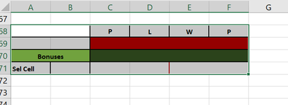
Please can you clarify the relevance of B2. The range A1:A5 is a column but I am looking for a range in is row (C123:F123) in my example.

The screen print shows the range as C68:F68 and the target cell is B71, but as mentioned I need to replicate this for multiple ranges and target cells.